Excel Conditional Formatting Whole Row

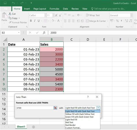
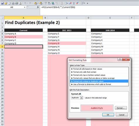
Excel conditional formatting is a powerful tool that allows users to highlight cells based on specific conditions, making it easier to analyze and understand data. One of the most useful applications of conditional formatting is highlighting entire rows based on the values in a specific column. This feature can be particularly helpful in identifying trends, patterns, or outliers in a dataset.

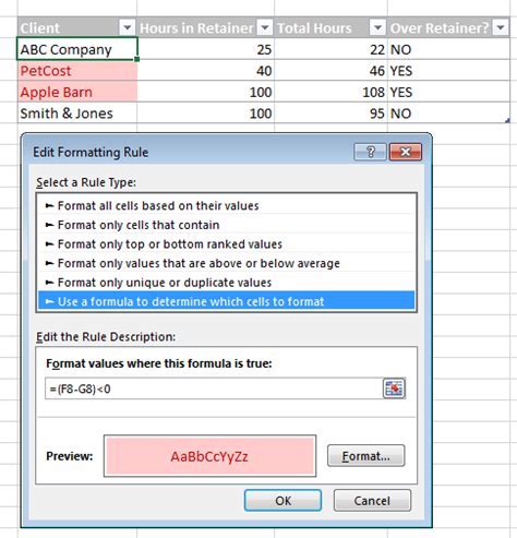
Conditional formatting can be applied to a whole row in Excel by using the "Format values where this formula is true" option in the conditional formatting rules. This method provides flexibility and allows users to create custom rules based on various conditions, including numerical values, text, and formulas.

To apply conditional formatting to a whole row in Excel, follow these steps:

Select the range of cells that you want to format, including the entire row.
Go to the "Home" tab in the Excel ribbon.
Click on the "Conditional Formatting" button in the "Styles" group.
Select "New Rule" from the dropdown menu.
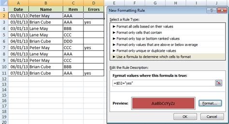
Choose the "Use a formula to determine which cells to format" option.
Enter a formula that refers to the cell in the column you want to base the formatting on. For example, if you want to highlight rows where the value in column A is greater than 10, you would enter =$A1>10.
Click on the "Format" button to select the formatting options you want to apply, such as fill color, font color, and border style.
Click "OK" to apply the rule.

Some examples of formulas that can be used to highlight entire rows based on specific conditions include:

=$A1>10 to highlight rows where the value in column A is greater than 10.
=$A1="Yes" to highlight rows where the value in column A is "Yes".
=ISBLANK($A1) to highlight rows where the value in column A is blank.

Benefits of Conditional Formatting

Conditional formatting offers several benefits, including:

Improved data visualization: Conditional formatting makes it easier to visualize data and identify patterns, trends, and outliers.
Enhanced analysis: By highlighting specific conditions, conditional formatting enables users to focus on the most important data and make more informed decisions.
Increased productivity: Conditional formatting saves time and effort by automating the process of highlighting cells based on specific conditions.

Common Use Cases for Conditional Formatting

Conditional formatting has a wide range of applications, including:

Highlighting due dates or deadlines
Identifying trends or patterns in data
Flagging errors or inconsistencies
Visualizing data distributions or correlations
Creating dashboards or reports

Some examples of industries or professions that can benefit from conditional formatting include:

Finance: to highlight changes in stock prices or identify trends in financial data
Marketing: to track website traffic or identify patterns in customer behavior
Healthcare: to monitor patient data or identify trends in disease outbreaks
Education: to track student performance or identify areas where students need improvement

Common Use Cases for Conditional Formatting

Advanced Conditional Formatting Techniques

Excel offers several advanced conditional formatting techniques, including:

Using multiple conditions: to highlight cells based on multiple conditions, such as values in multiple columns.
Using formulas: to create custom rules based on formulas, such as averaging values or calculating percentages.
Using formatting options: to apply different formatting options, such as fill color, font color, and border style.

Some examples of advanced conditional formatting techniques include:

Using the AND or OR functions to combine multiple conditions
Using the AVERAGE or PERCENTAGE functions to calculate values
Using the FORMAT function to apply custom formatting options

Best Practices for Conditional Formatting

To get the most out of conditional formatting, follow these best practices:

Keep it simple: avoid using complex formulas or conditions that can be difficult to understand.
Use clear and consistent formatting: use consistent formatting options throughout your worksheet to make it easier to understand.
Test and refine: test your conditional formatting rules and refine them as needed to ensure they are working correctly.

Some examples of best practices for conditional formatting include:

Using descriptive names for your rules
Using consistent formatting options throughout your worksheet
Testing your rules with sample data

Common Mistakes to Avoid

When using conditional formatting, avoid the following common mistakes:

Using absolute references: instead of using absolute references, such as $A$1, use relative references, such as A1.
Not testing your rules: test your conditional formatting rules with sample data to ensure they are working correctly.
Not using clear and consistent formatting: use consistent formatting options throughout your worksheet to make it easier to understand.

Some examples of common mistakes to avoid include:

Using the wrong formula or condition
Not applying the rule to the correct range of cells
Not using the correct formatting options

Gallery of Conditional Formatting Examples

Conditional Formatting Image Gallery

Another Example of Conditional Formatting

Different Example of Conditional Formatting

Example of Conditional Formatting with Multiple Conditions

Example of Conditional Formatting with Formulas

Example of Conditional Formatting with Formatting Options

Example of Conditional Formatting with Best Practices

Example of Conditional Formatting with Common Mistakes

Example of Conditional Formatting with Advanced Techniques

Example of Conditional Formatting with Real-World Applications

What is conditional formatting in Excel?

Conditional formatting is a feature in Excel that allows users to highlight cells based on specific conditions, such as values, formulas, or formatting options.

How do I apply conditional formatting to a whole row in Excel?

To apply conditional formatting to a whole row in Excel, select the range of cells, go to the "Home" tab, click on "Conditional Formatting", select "New Rule", and choose the "Use a formula to determine which cells to format" option.

What are some common use cases for conditional formatting?

Some common use cases for conditional formatting include highlighting due dates or deadlines, identifying trends or patterns in data, flagging errors or inconsistencies, and visualizing data distributions or correlations.

How do I create custom rules for conditional formatting?

To create custom rules for conditional formatting, use the "Use a formula to determine which cells to format" option and enter a formula that refers to the cell in the column you want to base the formatting on.

What are some best practices for conditional formatting?

Some best practices for conditional formatting include keeping it simple, using clear and consistent formatting, and testing and refining your rules.

We hope this article has provided you with a comprehensive understanding of conditional formatting in Excel and how to apply it to a whole row. By following the steps and tips outlined in this article, you can create custom rules and formatting options to make your data more visual and easier to understand. If you have any further questions or need more assistance, please don't hesitate to ask. Share your experiences with conditional formatting in the comments below, and help others learn from your expertise.