Excel Drop Down List Colour

Creating a drop-down list in Excel can be a powerful tool for organizing and streamlining data entry. One of the key features that can enhance the usability and visual appeal of these lists is the ability to change their background color. This can help in distinguishing between different types of data, highlighting important information, or simply making your spreadsheet more visually appealing.

The importance of customization in Excel cannot be overstated. By allowing users to personalize their spreadsheets, including the colors of drop-down lists, Excel provides a more engaging and effective way to interact with data. Whether you're working on a personal project, a professional report, or an educational assignment, the ability to customize the appearance of your spreadsheet can make a significant difference in how information is perceived and understood.

For individuals and businesses alike, effective data presentation is crucial. It can mean the difference between a spreadsheet that is easy to navigate and understand, and one that is confusing and overwhelming. By incorporating visual elements such as color into your drop-down lists, you can create a more intuitive and user-friendly experience. This is particularly important in collaborative environments where clear and accessible data presentation can facilitate communication and decision-making.

Benefits of Customizing Drop Down List Colour

Customizing the color of a drop-down list in Excel offers several benefits. Firstly, it allows for better data differentiation, making it easier to categorize and identify specific types of information at a glance. Secondly, it can enhance the aesthetic appeal of your spreadsheet, making it more engaging and professional-looking. Lastly, color customization can play a crucial role in accessibility, helping users with visual impairments by providing high contrast colors that are easier to read.

How to Change the Colour of a Drop Down List

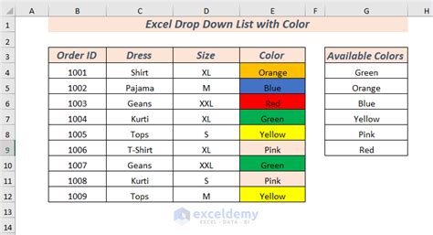
To change the color of a drop-down list in Excel, you can follow these steps: - Select the cell that contains the drop-down list. - Go to the "Home" tab on the Ribbon. - Click on the "Font" group and select the desired color from the color palette. - Alternatively, for more detailed color options, click on the "More Colors" button and choose from the available palette or enter a custom color code.

It's worth noting that while Excel provides extensive formatting options, including colors, for cells and text, the drop-down list itself is a product of data validation. The background color of the drop-down list is determined by the cell's formatting, but the list's appearance (such as the color of the list items) is more limited in terms of customization directly through Excel's built-in tools.

Working with Conditional Formatting

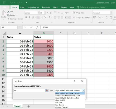
Conditional formatting is another powerful feature in Excel that can be used in conjunction with drop-down lists to create dynamic and interactive spreadsheets. By applying conditional formatting rules, you can change the appearance of cells based on specific conditions, such as the value of the cell, the value of another cell, or even the format of the cell (like font color, fill color, etc.).

To apply conditional formatting to a cell that contains a drop-down list:

• Select the cell or range of cells.
• Go to the "Home" tab and click on "Conditional Formatting".
• Choose the type of rule you want to apply (e.g., "Highlight Cells Rules", "Top/Bottom Rules", etc.).
• Select the specific formatting you wish to apply based on the condition.

This feature is particularly useful for highlighting important information, tracking trends, or identifying data that meets specific criteria, all of which can be tied back to the selection made from a drop-down list.

Steps to Create a Drop Down List

Creating a drop-down list in Excel involves using the data validation feature. Here are the steps to follow: 1. **Select the Cell**: Choose the cell where you want the drop-down list to appear. 2. **Data Validation**: Go to the "Data" tab on the Ribbon and click on "Data Validation". 3. **Settings**: In the Data Validation dialog box, under the "Settings" tab, select "List" from the "Allow" dropdown menu. 4. **Source**: Enter the range of cells that contains the list of items you want to appear in the drop-down list, or select the range directly in the worksheet. 5. **Apply**: Click "OK" to apply the data validation and create the drop-down list.

Practical Applications of Drop Down Lists

Drop-down lists have a wide range of practical applications in Excel, from simplifying data entry to enhancing data analysis. Some key uses include:

• Data Entry: Reducing errors by limiting input to a predefined list of options.
• Surveys and Forms: Creating interactive forms where users can select from a list of options.
• Dashboards: Enhancing the visual appeal and interactivity of dashboards by allowing users to select different data views or parameters.

By combining drop-down lists with other Excel features, such as macros, pivot tables, and conditional formatting, you can create sophisticated and dynamic spreadsheets that are both functional and visually appealing.

Common Challenges and Solutions

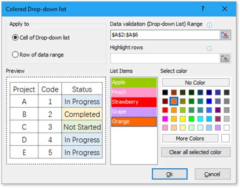
When working with drop-down lists in Excel, users may encounter several challenges, including: - **Limited List Size**: Excel has limitations on the number of items that can be displayed in a drop-down list. To overcome this, consider using a separate worksheet for the list and referencing it. - **Dynamic Lists**: Creating lists that update automatically based on other data in the spreadsheet. This can be achieved using formulas like OFFSET and COUNTA to dynamically define the list range.

Gallery of Excel Drop Down List Colour Customization

Excel Drop Down List Colour Customization Gallery

Frequently Asked Questions

How do I create a drop-down list in Excel?

+

To create a drop-down list, select the cell, go to the Data tab, click on Data Validation, select List, and then specify the source range.

Can I change the color of the drop-down list in Excel?

+

Yes, you can change the background color of the cell that contains the drop-down list, which will also change the appearance of the list when it's displayed.

How do I apply conditional formatting to a cell with a drop-down list?

+

Select the cell, go to the Home tab, click on Conditional Formatting, choose a rule type, and then apply the desired formatting based on your conditions.

In conclusion, customizing the color of a drop-down list in Excel, along with leveraging other features like conditional formatting, can significantly enhance the usability and visual appeal of your spreadsheets. Whether you're a professional analyst, a student, or simply someone looking to organize personal data more effectively, understanding how to work with drop-down lists and customize their appearance can make a substantial difference in how you interact with and present data in Excel. We invite you to share your experiences, tips, and questions about working with drop-down lists and color customization in Excel in the comments below.