Highlight Cells Greater Than

Highlighting cells that contain values greater than a specific number is a common task in data analysis, particularly when working with spreadsheets like Microsoft Excel or Google Sheets. This feature helps in quickly identifying important data points, such as high scores, large quantities, or significant values, that stand out from the rest. Let's dive into how to achieve this in both Excel and Google Sheets, as well as explore some advanced techniques for more complex data analysis.

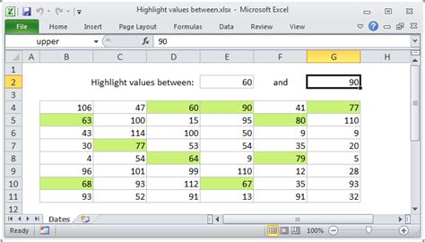
When you're dealing with a large dataset, being able to visually distinguish between different values can greatly enhance your understanding and interpretation of the data. Highlighting cells based on conditions such as being greater than a certain value is not only useful for initial data exploration but also for presenting findings in a clear and compelling way.

Why Highlight Cells Greater Than a Specific Value?

Highlighting cells greater than a specific value can serve several purposes:

• Data Visualization: It helps in creating a visual representation of your data, making it easier to understand and analyze.
• Identification of Outliers: High values can sometimes indicate outliers or anomalies in the data that may require further investigation.
• Prioritization: In business or project management, highlighting high-priority tasks or large quantities can aid in decision-making and resource allocation.
• Quality Control: In manufacturing or quality control, identifying values that exceed certain thresholds can be crucial for ensuring product quality and safety.

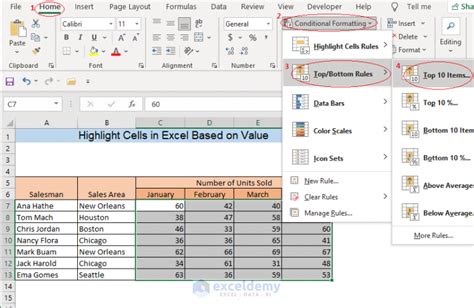
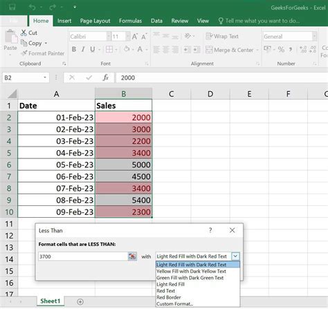
How to Highlight Cells in Excel

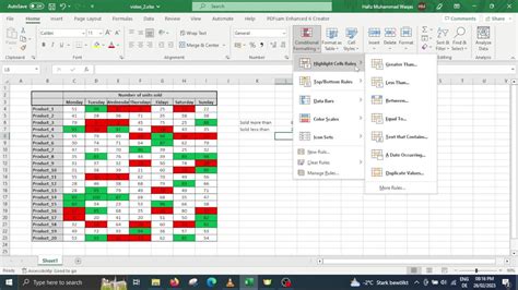
Microsoft Excel provides a straightforward method to highlight cells based on specific conditions, including values greater than a certain number. Here’s how you can do it:

1. Select the range of cells you want to format.
2. Go to the "Home" tab on the Ribbon.
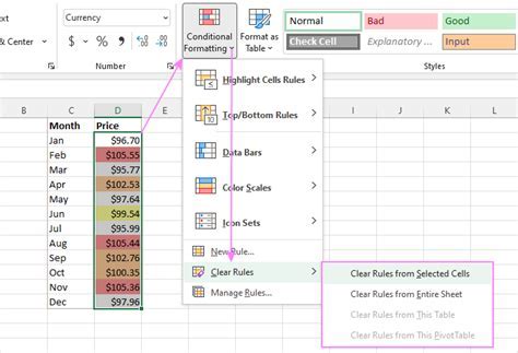
3. Click on "Conditional Formatting" in the Styles group.
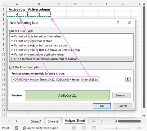
4. Choose "New Rule."
5. Select "Use a formula to determine which cells to format."
6. Enter a formula like =A1>10 if you want to highlight cells greater than 10 in column A.
7. Click "Format" to choose how you want to highlight the cells (e.g., fill color, font color).
8. Click "OK" to apply the rule.

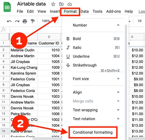
How to Highlight Cells in Google Sheets

Google Sheets also offers a similar functionality:

1. Select the cells you want to format.
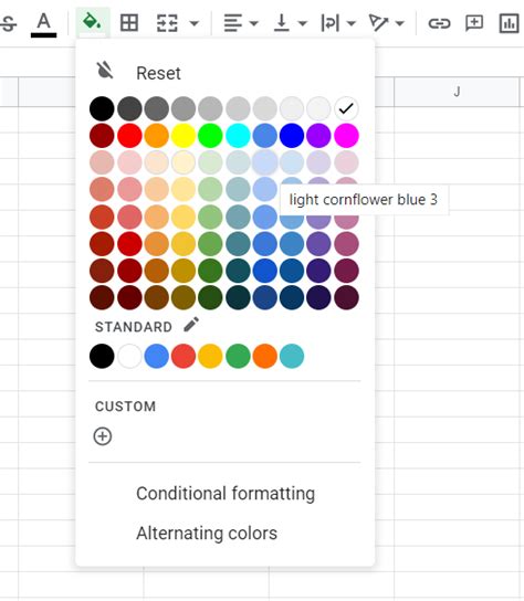
2. Go to the "Format" tab.
3. Hover over "Conditional formatting."
4. Choose "Custom formula is" from the format cells if dropdown.
5. Enter a formula like =A1>10 for cells in column A greater than 10.
6. Choose the formatting you want to apply.
7. Click "Done."

Advanced Techniques for Conditional Formatting

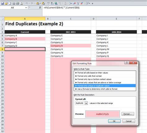
Beyond simple comparisons, you can use more complex formulas to highlight cells based on multiple conditions or relative references. For example, using the AND or OR functions can help you highlight cells that meet more than one condition.

Using AND and OR Functions

• AND Function: =AND(A1>10, B1="Yes") highlights cells in A1 if the value is greater than 10 and the corresponding cell in B1 contains "Yes."
• OR Function: =OR(A1>10, B1="Yes") highlights cells if either condition is true.

Highlighting Cells Based on Relative References

Using relative references (like A1) in your formulas allows the conditional formatting to adjust to each cell in the selected range, making the rule apply correctly across different cells.

Best Practices for Highlighting Cells

• Keep it Simple: Avoid overly complex rules that might be hard to understand or maintain.
• Use Clear Formatting: Ensure the highlighting is clear and distinguishable from other formatting in your spreadsheet.
• Test Your Rules: Always test your conditional formatting rules on a small set of data before applying them to larger datasets.

Common Mistakes to Avoid

• Incorrect References: Double-check that your formulas reference the correct cells or ranges.
• Formula Errors: Make sure your formulas are syntactically correct and logically sound.
• Overlapping Rules: Be cautious of creating rules that overlap or conflict with each other.

Conclusion and Next Steps

Highlighting cells greater than a specific value is a powerful tool for data analysis and visualization. By mastering conditional formatting in Excel and Google Sheets, you can enhance your data analysis capabilities, make your spreadsheets more intuitive, and present your findings more effectively. Remember to keep your rules simple, test them thoroughly, and avoid common pitfalls to get the most out of this feature.

Gallery of Highlighting Cells Greater Than a Specific Value

Highlighting Cells Image Gallery

FAQs

What is conditional formatting in Excel and Google Sheets?

+

Conditional formatting is a feature that allows you to apply formatting to a cell or range of cells based on specific conditions or criteria.

How do I highlight cells greater than a specific value in Excel?

+

To highlight cells greater than a specific value in Excel, use the conditional formatting feature with a formula like =A1>10 for cells in column A.

Can I use conditional formatting in Google Sheets?

+

Yes, Google Sheets supports conditional formatting. You can access it through the Format tab and then select Conditional formatting.

If you have any questions or need further assistance with highlighting cells greater than a specific value in Excel or Google Sheets, don't hesitate to ask. Share your experiences or tips on using conditional formatting for data analysis and visualization in the comments below.