How To Show Min Max And Average In Excel Graph

Understanding how to effectively display data in Excel graphs is crucial for data analysis and presentation. One common requirement is to show minimum, maximum, and average values in an Excel graph. This can help in visually identifying trends, outliers, and the central tendency of the data. Let's dive into the steps and methods to achieve this.

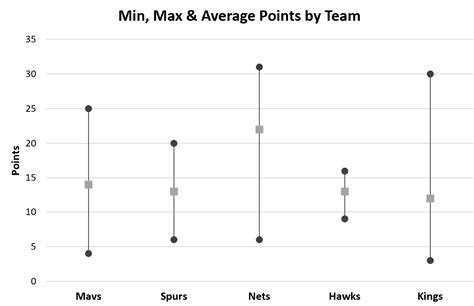
Displaying minimum, maximum, and average values on a graph can significantly enhance the readability and usefulness of the data visualization. It provides immediate insights into the range of values (through min and max) and the central tendency (through average). This is particularly useful in comparative analyses, trend analyses, and when trying to understand the distribution of data points.

Introduction to Excel Graphs

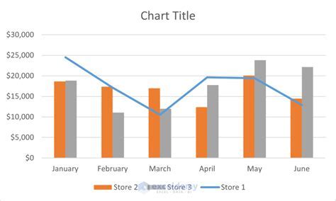
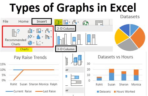
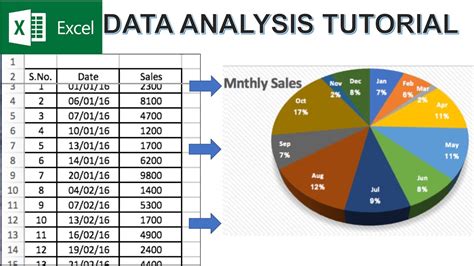
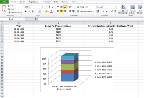
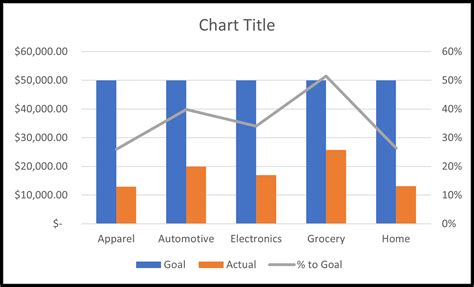
Excel offers a variety of graph types, including line graphs, column graphs, pie charts, and more. Each type of graph is suited for different kinds of data and analysis needs. For showing min, max, and average values, column graphs or line graphs are often the most effective.

Preparing Your Data

Before creating a graph, it's essential to have your data well-organized. Typically, this means having your data in a table format with headers in the first row and data points below. If you're calculating min, max, and average, you might have separate columns for these calculations. Excel formulas like MIN(range), MAX(range), and AVERAGE(range) can be used to calculate these values.

Creating a Basic Graph

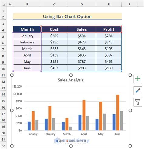
1. Select the data range you want to graph, including headers.
2. Go to the "Insert" tab on the ribbon.
3. Choose the type of graph you want (e.g., 2D Column).
4. Click on the graph type to insert it into your worksheet.

Adding Min, Max, and Average to the Graph

To add min, max, and average lines to your graph, you can use the following methods:

Method 1: Using Calculated Fields

1. Select your graph.
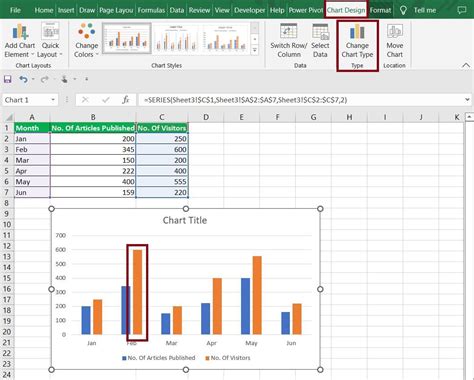
2. Go to the "Chart Design" tab.
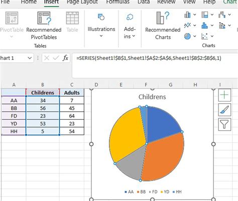
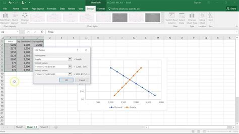
3. Click on "Select Data".
4. Click "Add" to add a new series for min, max, or average.
5. In the series name, reference the cell with your min, max, or average formula.
6. For series values, select the range of cells containing the calculated min, max, or average values.

Method 2: Using Error Bars

For showing min and max values as error bars around an average line:

1. Select the series that represents your average.
2. Go to the "Chart Design" tab.
3. Click on "Add Chart Element" and select "Error Bars".
4. Choose "Custom" and then select the ranges for your min and max values.

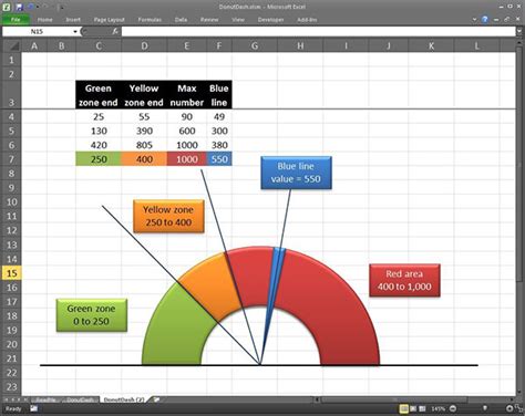
Customizing Your Graph

After adding min, max, and average to your graph, you may want to customize the appearance. This can include changing colors, adding labels, or modifying the axis scales. The "Chart Design" and "Format" tabs offer a range of tools for customization.

Interpreting the Graph

Once your graph is set up, you can use it to analyze your data. Look for:

• Trends: How data points change over time or categories.
• Outliers: Data points that are significantly higher or lower than the average.
• Range: The difference between max and min values gives you the range of your data.

Common Challenges and Solutions

• Data Not Displaying Correctly: Check that your data range is correctly selected and that there are no blank rows or columns in your data.
• Graph Not Updating: Ensure that your graph is linked to the correct data range and that calculations for min, max, and average are updating automatically.

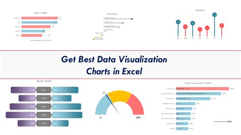
Excel Graph Gallery

How do I select the right type of graph for my data?

+

The type of graph depends on the nature of your data and what you want to show. For example, use a line graph for trends over time, a column graph for comparing categories, and a pie chart for showing parts of a whole.

Can I customize the appearance of my graph?

+

Yes, Excel offers a wide range of customization options for graphs, including changing colors, fonts, adding labels, and modifying axis scales. Use the "Chart Design" and "Format" tabs to make these changes.

How do I add a trendline to my graph?

+

To add a trendline, select your graph, go to the "Chart Design" tab, click on "Add Chart Element", and choose "Trendline". Then, select the type of trendline you want, such as linear or exponential.

In conclusion, showing min, max, and average values in an Excel graph is a powerful way to enhance data visualization and analysis. By following the steps outlined above and customizing your graph as needed, you can create effective and informative graphs that help in understanding and presenting your data. Remember, the key to a good graph is clarity, simplicity, and relevance to your analysis goals. Whether you're a beginner or an advanced user, mastering Excel graphs can significantly improve your data analysis capabilities.