Google Sheets Conditional Formatting Highlight Row If Cell Contains Text

Google Sheets is a powerful tool for data analysis and management, offering a wide range of features to help users organize, visualize, and understand their data. One of these features is conditional formatting, which allows users to apply specific formatting to cells based on the values or formulas they specify. Highlighting rows if a cell contains specific text is one common use of conditional formatting that can help draw attention to important information, categorize data, or simply make a spreadsheet more readable.

Conditional formatting in Google Sheets is straightforward to apply and can be customized to fit various needs. Here's a step-by-step guide on how to highlight a row if a cell contains specific text:

Step 1: Select the Range

First, you need to select the range of cells you want to apply the formatting to. This could be an entire column, a row, or a specific group of cells. For example, if you want to highlight rows based on the content of column A, select the entire range (e.g., A1:Z1000, assuming your data is within the first 1000 rows and you want to consider all columns up to Z).

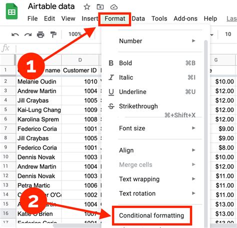
Step 2: Open Conditional Formatting

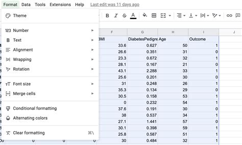
With your range selected, go to the "Format" tab in the menu. From the dropdown menu, select "Conditional formatting." This will open the conditional formatting sidebar where you can set up your rules.

Step 3: Set Up the Rule

In the conditional formatting sidebar, you'll see a few options:

• Format cells if: This is where you specify the condition. For highlighting rows based on text, select "Custom formula is".
• Format values where this formula is true: Here, you will enter a formula that checks if a cell contains specific text. For example, if you want to highlight rows where the cell in column A contains the word "Example", your formula would be =REGEXMATCH(A1, "Example").
  • Note: A1 refers to the first cell in your selected range. The formula automatically applies to the entire range you've selected.
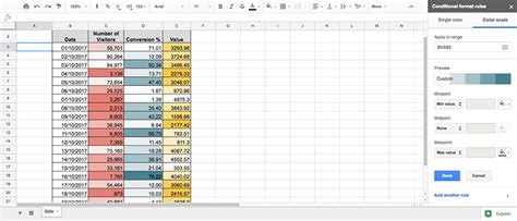
• Format: Choose how you want the row to be highlighted (e.g., fill color, font color).

Step 4: Apply to Entire Row

By default, conditional formatting only applies to the selected cells. To make it apply to the entire row:

• Check the box that says "Format entire row" at the bottom of the formatting options sidebar.

Step 5: Done

Click "Done" to apply your rule. Google Sheets will now highlight any row where the specified condition is met.

Tips and Variations

• Case Sensitivity: The REGEXMATCH function is case-sensitive. If you want a case-insensitive match, you can modify your formula like this: =REGEXMATCH(A1, "Example", "i").
• Multiple Conditions: You can also highlight rows based on multiple conditions by using the OR or AND functions in your formula. For example, to highlight rows where column A contains either "Example1" or "Example2", you could use =OR(REGEXMATCH(A1, "Example1"), REGEXMATCH(A1, "Example2")).
• Applying to Other Columns: If you want to apply the formatting based on a column other than the one you're looking at, just adjust the column letter in your formula accordingly.

Common Use Cases

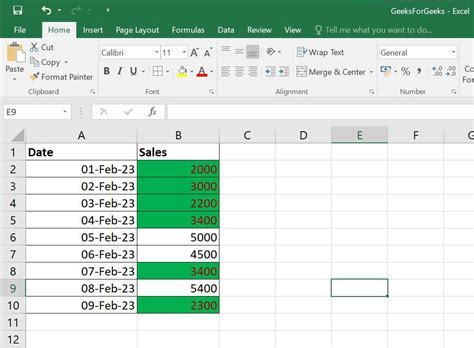
• Data Filtering: Highlighting specific data points can help in quickly identifying trends or outliers in your dataset.
• Task Management: In a task list, you might highlight rows where the status is "Urgent" or "Overdue".
• Inventory Management: Highlighting items that are out of stock or near the reorder point can help in managing inventory levels efficiently.

Troubleshooting

• Formula Errors: Ensure your formula is correctly written and references the correct cells or columns.
• No Formatting Applied: Check that your condition is met in at least one row and that the "Format entire row" option is selected if you want the whole row to be highlighted.

Conclusion and Next Steps

Conditional formatting is a powerful feature in Google Sheets that can significantly enhance your data analysis and presentation capabilities. By mastering how to highlight rows based on specific text, you can make your spreadsheets more informative and easier to navigate. Experiment with different formulas and formatting options to find the methods that work best for your specific needs. Whether you're managing a simple to-do list or complex datasets, leveraging conditional formatting can take your spreadsheet game to the next level.

Advanced Conditional Formatting Techniques

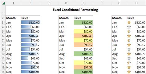
For those looking to dive deeper into what conditional formatting can offer, there are several advanced techniques worth exploring. These include using custom formulas to apply formatting based on complex conditions, leveraging the INDIRECT function to dynamically reference ranges, and creating custom color scales to visually represent data trends.

Best Practices for Using Conditional Formatting

While conditional formatting is a powerful tool, it's essential to use it judiciously to avoid overwhelming your spreadsheet with too much visual information. Best practices include limiting the number of formatting rules, using consistent formatting throughout the spreadsheet, and regularly reviewing and updating your rules as your data evolves.

Common Conditional Formatting Mistakes

Even experienced users can fall into traps when applying conditional formatting. Common mistakes include forgetting to update the applied range when adding new data, using formulas that are too complex or inefficient, and not testing the formatting rules thoroughly before applying them to large datasets.

Conditional Formatting for Data Analysis

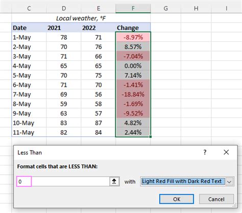
Conditional formatting is not just about making your spreadsheet look pretty; it's a critical tool for data analysis. By highlighting trends, outliers, and patterns, you can gain deeper insights into your data, make more informed decisions, and present your findings more effectively.

Gallery of Conditional Formatting Examples

Conditional Formatting Image Gallery

Frequently Asked Questions

What is conditional formatting in Google Sheets?

+

Conditional formatting is a feature that allows you to apply specific formatting to cells based on the values or formulas you specify.

How do I highlight an entire row based on a condition?

+

Select the range, go to Format > Conditional formatting, set your condition, and check the box that says "Format entire row" at the bottom of the formatting options sidebar.

Can I use conditional formatting with multiple conditions?

+

Yes, you can use the OR or AND functions in your formula to apply formatting based on multiple conditions.

If you've made it this far, congratulations! You're well on your way to becoming a master of Google Sheets conditional formatting. Whether you're a beginner looking to enhance your spreadsheet skills or an advanced user seeking to refine your techniques, the world of conditional formatting has something to offer. Share your thoughts, ask questions, or showcase your conditional formatting creations in the comments below. Let's keep the conversation going and explore the endless possibilities that Google Sheets has to offer.