How To Filter Multiple Colored Cells In Excel

The ability to filter multiple colored cells in Excel can be a powerful tool for data analysis and visualization. Excel's built-in filtering capabilities allow users to quickly and easily narrow down their data to specific criteria, including cell color. This feature can be particularly useful when working with large datasets where color-coding has been used to highlight important information, trends, or patterns.

Excel's conditional formatting feature is often used to apply different colors to cells based on specific conditions, such as values, formulas, or formatting. However, the default filtering options in Excel do not directly support filtering by cell color. Fortunately, there are several workarounds and methods that can be employed to filter multiple colored cells in Excel.

To begin with, it's essential to understand the basics of Excel filtering and how to apply conditional formatting to cells. Excel's filtering feature allows users to select specific data to display, hiding the rest of the data. This can be done using the "Filter" button in the "Data" tab of the ribbon. Conditional formatting, on the other hand, enables users to apply different formats to cells based on specific conditions.

Understanding Conditional Formatting

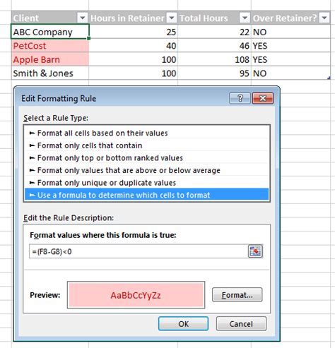
Conditional formatting is a powerful feature in Excel that allows users to apply different formats to cells based on specific conditions. This can include formatting cells based on their values, formulas, or formatting. To apply conditional formatting, users can select the cells they want to format, go to the "Home" tab, and click on the "Conditional Formatting" button in the "Styles" group.

Types of Conditional Formatting

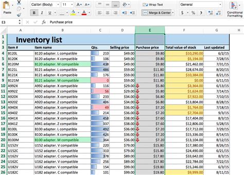
There are several types of conditional formatting available in Excel, including: * Highlight Cells Rules: This type of formatting allows users to highlight cells based on specific conditions, such as values, formulas, or formatting. * Top/Bottom Rules: This type of formatting allows users to highlight cells that are in the top or bottom percentage of a selected range. * Data Bars: This type of formatting allows users to display data bars in cells to represent the value of the cell. * Color Scales: This type of formatting allows users to apply color scales to cells to represent the value of the cell. * Icon Sets: This type of formatting allows users to apply icon sets to cells to represent the value of the cell.

Filtering Multiple Colored Cells

Filtering multiple colored cells in Excel can be done using several methods, including:

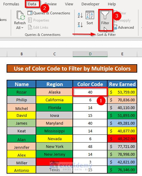
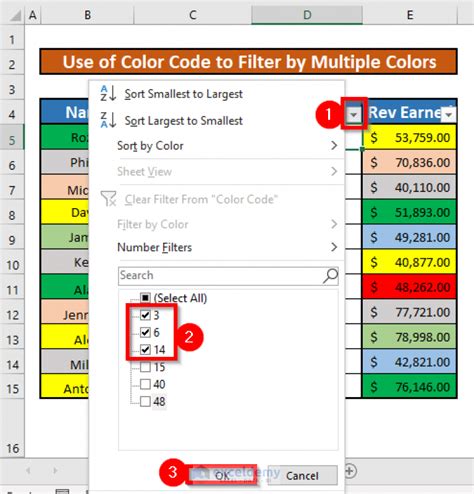
Using the "Filter" button: Users can select the cells they want to filter, go to the "Data" tab, and click on the "Filter" button. Then, they can select the "Filter by Color" option and choose the color they want to filter by.
Using a pivot table: Users can create a pivot table and use the "Filter" option to filter the data by color.
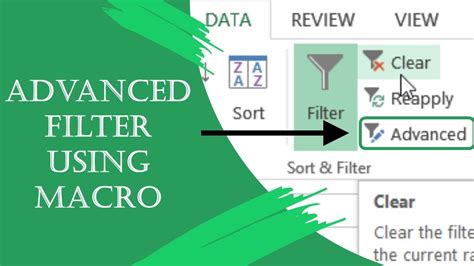
Using a macro: Users can create a macro to filter the data by color.

Step-by-Step Guide to Filtering Multiple Colored Cells

Here is a step-by-step guide to filtering multiple colored cells in Excel: 1. Select the cells you want to filter. 2. Go to the "Data" tab and click on the "Filter" button. 3. Select the "Filter by Color" option and choose the color you want to filter by. 4. Click "OK" to apply the filter.

Using VBA to Filter Multiple Colored Cells

VBA (Visual Basic for Applications) is a powerful programming language that can be used to automate tasks in Excel. Users can create a VBA macro to filter multiple colored cells in Excel. Here is an example of a VBA macro that filters multiple colored cells:

Sub FilterByColor()
    Dim rng As Range
    Set rng = Selection
    For Each cell In rng
        If cell.Interior.ColorIndex = 3 Then
            cell.EntireRow.Hidden = False
        Else
            cell.EntireRow.Hidden = True
        End If
    Next cell
End Sub

This macro filters the selected cells by color and hides the rows that do not match the color.

Benefits of Using VBA to Filter Multiple Colored Cells

Using VBA to filter multiple colored cells has several benefits, including: * Increased efficiency: VBA macros can automate tasks and increase efficiency. * Flexibility: VBA macros can be customized to meet specific needs. * Accuracy: VBA macros can reduce errors and improve accuracy.

Gallery of Excel Filtering Techniques

Excel Filtering Techniques Image Gallery

Frequently Asked Questions

What is conditional formatting in Excel?

Conditional formatting is a feature in Excel that allows users to apply different formats to cells based on specific conditions.

How do I filter multiple colored cells in Excel?

To filter multiple colored cells in Excel, users can select the cells they want to filter, go to the "Data" tab, and click on the "Filter" button. Then, they can select the "Filter by Color" option and choose the color they want to filter by.

Can I use VBA to filter multiple colored cells in Excel?

Yes, users can create a VBA macro to filter multiple colored cells in Excel. This can be done by recording a macro or writing a custom macro using VBA code.

In conclusion, filtering multiple colored cells in Excel can be a powerful tool for data analysis and visualization. By using conditional formatting, filtering, and VBA macros, users can quickly and easily narrow down their data to specific criteria, including cell color. Whether you're a beginner or an advanced user, mastering these techniques can help you to work more efficiently and effectively with your data. So, take the time to explore these features and discover how they can help you to unlock the full potential of your data. We invite you to share your experiences, ask questions, or provide feedback on this topic in the comments section below.