Intro
Learn to keep row headings visible in Excel when scrolling, using freeze panes, formulas, and other techniques to enhance spreadsheet navigation and data analysis with column headers and row labels.
When working with large datasets in Excel, it can be frustrating to lose sight of the column headers as you scroll down through the rows. This can make it difficult to understand the context of the data and can lead to errors. Fortunately, Excel provides a few ways to keep the row headings visible while scrolling.
Freezing panes is one of the most common methods used to keep row headings visible. This feature allows you to lock specific rows or columns in place, so they remain visible even when you scroll through the rest of the worksheet. To freeze the top row, which typically contains the column headers, you can use the "Freeze Panes" option in the "View" tab of the ribbon.
Another method is to use the "Split" feature, which divides the worksheet into separate panes that can be scrolled independently. This allows you to keep the row headings visible in one pane while scrolling through the data in another. The "Split" feature can be accessed from the "View" tab of the ribbon, and you can adjust the position of the split by dragging the split bar.
Using a table with headers is another way to keep row headings visible. When you convert a range of cells to a table, Excel automatically adds filters and formatting to the headers. The headers will also remain visible when you scroll through the table, making it easier to understand the data.
In addition to these methods, you can also use the "Page Layout View" to keep row headings visible. This view allows you to see the worksheet as it will be printed, with the row headings repeated at the top of each page. You can access the "Page Layout View" from the "View" tab of the ribbon.
Overall, keeping row headings visible while scrolling is an important feature in Excel that can help you work more efficiently and accurately with large datasets. By using one of the methods described above, you can ensure that the row headings remain visible, making it easier to understand and analyze the data.
Freezing Panes in Excel
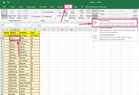
To freeze the top row, select the row below the headers, go to the "View" tab, and click on "Freeze Panes." Then, select "Freeze Panes" again, and choose "Freeze Top Row." This will lock the top row in place, so it remains visible even when you scroll through the rest of the worksheet.
Benefits of Freezing Panes
Freezing panes has several benefits, including: * Keeping column headers visible while scrolling through large datasets * Making it easier to understand the context of the data * Reducing errors caused by losing sight of the column headers * Improving productivity by allowing you to work more efficiently with large datasetsSplitting the Worksheet
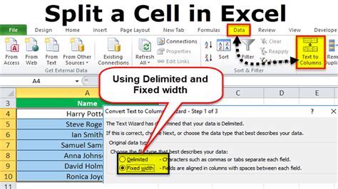
To split the worksheet, go to the "View" tab, and click on "Split." This will divide the worksheet into four panes, each of which can be scrolled independently. You can adjust the position of the split by dragging the split bar, which allows you to customize the layout of the worksheet.
Benefits of Splitting the Worksheet
Splitting the worksheet has several benefits, including: * Keeping row headings visible while scrolling through large datasets * Allowing you to compare data from different parts of the worksheet * Improving productivity by allowing you to work more efficiently with large datasets * Making it easier to understand the context of the dataUsing a Table with Headers
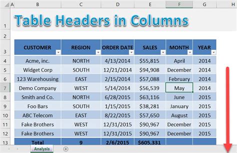
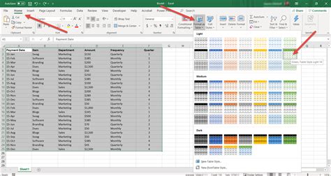
To convert a range of cells to a table, select the range, go to the "Insert" tab, and click on "Table." This will open the "Create Table" dialog box, where you can choose the range of cells to include in the table. Once you have created the table, you can customize the headers by adding filters, formatting, and other features.
Benefits of Using a Table with Headers
Using a table with headers has several benefits, including: * Keeping row headings visible while scrolling through large datasets * Making it easier to understand the context of the data * Improving productivity by allowing you to work more efficiently with large datasets * Allowing you to filter and sort the data more easilyPage Layout View
To access Page Layout View, go to the "View" tab, and click on "Page Layout View." This will display the worksheet as it will be printed, with the row headings repeated at the top of each page. You can customize the layout of the page by adjusting the margins, headers, and footers.
Benefits of Page Layout View
Page Layout View has several benefits, including: * Allowing you to see the worksheet as it will be printed * Making it easier to understand the context of the data * Improving productivity by allowing you to work more efficiently with large datasets * Allowing you to customize the layout of the pageExcel Image Gallery

How do I freeze panes in Excel?
+To freeze panes in Excel, select the row below the headers, go to the "View" tab, and click on "Freeze Panes." Then, select "Freeze Panes" again, and choose "Freeze Top Row."
How do I split the worksheet in Excel?
+To split the worksheet in Excel, go to the "View" tab, and click on "Split." This will divide the worksheet into four panes, each of which can be scrolled independently.
How do I use a table with headers in Excel?
+To use a table with headers in Excel, select the range of cells, go to the "Insert" tab, and click on "Table." This will open the "Create Table" dialog box, where you can choose the range of cells to include in the table.
We hope this article has provided you with useful tips and tricks for keeping row headings visible while scrolling in Excel. Whether you're working with large datasets or just need to keep your column headers visible, these methods can help you work more efficiently and accurately. If you have any questions or comments, please don't hesitate to share them with us. We'd love to hear from you and help you get the most out of Excel.