Apply Conditional Formatting Entire Row Google Sheets

The ability to apply conditional formatting to an entire row in Google Sheets can greatly enhance the visual organization and readability of your data. This feature allows you to highlight rows based on specific conditions, making it easier to identify patterns, trends, or specific data points of interest. Here's how you can apply conditional formatting to entire rows in Google Sheets, along with examples and tips to get the most out of this feature.

First, let's understand why conditional formatting is useful. It helps in drawing attention to important information, such as deadlines, targets, or anomalies in your data. By applying formatting rules to entire rows, you can quickly scan your spreadsheet and focus on the data that matters most.

To apply conditional formatting to an entire row in Google Sheets, follow these steps:

Select the Range: Start by selecting the range of cells that you want to apply the conditional formatting to. If you want to format entire rows based on a condition, select the column that contains the values you want to base your condition on.
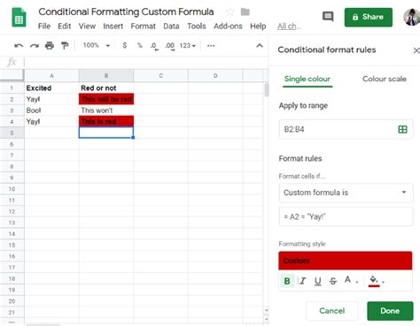
Open Conditional Format Rules: Go to the "Format" tab in the menu, hover over "Conditional formatting," and click on it. This will open the conditional format rules sidebar.
Set Up Your Rule: In the format cells if dropdown, select the condition you want to apply (e.g., "Custom formula is").
Apply to Entire Row: To apply the formatting to the entire row, you will use a custom formula. For example, if you want to highlight rows where the value in column A is greater than 10, you would use the formula =A1>10. However, to apply this rule to the entire row, you need to adjust the formula to reference the entire row. Since Google Sheets automatically applies the rule to each cell in the selected range, you can simply use a formula that references the first cell of each row and it will be applied across the row.
Format: Choose how you want to format the cells (e.g., background color, text color).
Done: Click "Done" to apply your rule.

Here's a more detailed example:

Suppose you have a spreadsheet with student names in column A, their ages in column B, and their scores in column C. You want to highlight the entire row for students who scored above 80.

Select column A (or the entire range if you prefer, A:C for example).
Go to "Format" > "Conditional formatting".
In the format cells if dropdown, select "Custom formula is".
Enter the formula: =C1>80 (assuming your data starts from row 1).
Choose your formatting (e.g., fill background with a specific color).
Click "Done".

Google Sheets will now highlight the entire row for any student who scored above 80, based on the value in column C.

Conditional formatting rows in Google Sheets

Advanced Conditional Formatting

For more complex conditions, you can use combinations of functions like AND, OR, and NOT within your custom formulas. For example, to highlight rows where the score is above 80 and the age is greater than 18, you could use:

=AND(C1>80, B1>18)

This formula checks both conditions (score > 80 and age > 18) and only applies the formatting if both are true.

Formatting Based on Other Columns

If you want to format rows based on conditions in other columns, simply adjust your formula to reference those columns. For instance, to format rows based on values in column D, your formula might look like =D1>10.

Common Use Cases

Highlighting Due Dates: Use conditional formatting to highlight rows where a project is due soon or overdue based on the current date.
Identifying Trends: Apply formatting to show trends in your data, such as increases or decreases in sales over time.
Flagging Anomalies: Use conditional formatting to quickly identify data points that are significantly different from the rest, such as unusually high or low values.

Examples of conditional formatting in Google Sheets

Troubleshooting

Formula Errors: If your formula is not working as expected, check for syntax errors or ensure that the formula is correctly referencing the cells or columns you intend.
Formatting Not Applying: Make sure the range you've selected matches the range you want to format. Also, check if there are any overlapping rules that might be interfering with your intended formatting.

Best Practices for Conditional Formatting

Keep It Simple: Avoid overly complex formulas that can be hard to understand or debug.
Use Clear and Consistent Formatting: Choose formats that are easy to distinguish and apply them consistently across your spreadsheet.
Test Your Rules: Before applying rules to large datasets, test them on a small sample to ensure they work as expected.

Best practices for using conditional formatting

Gallery of Conditional Formatting Examples

Conditional Formatting Image Gallery

What is conditional formatting in Google Sheets?

Conditional formatting is a feature in Google Sheets that allows you to automatically format cells based on the data they contain. This can include highlighting cells that meet certain conditions, such as being greater than a certain value, containing specific text, or being within a certain date range.

How do I apply conditional formatting to an entire row in Google Sheets?

To apply conditional formatting to an entire row, select the range of cells you want to format, go to the "Format" tab, select "Conditional formatting," and then choose the condition you want to apply. Use a custom formula that references the first cell of each row to apply the formatting across the entire row.

Can I use conditional formatting with other Google Sheets functions?

Yes, conditional formatting can be used in conjunction with other Google Sheets functions, such as filtering, sorting, and pivot tables, to create powerful and dynamic spreadsheets that help you analyze and understand your data more effectively.

In conclusion, applying conditional formatting to entire rows in Google Sheets is a powerful tool for data analysis and visualization. By following the steps and tips outlined above, you can unlock the full potential of conditional formatting and take your spreadsheet skills to the next level. Whether you're a beginner or an advanced user, mastering conditional formatting can help you work more efficiently and make better decisions based on your data. So, start exploring the world of conditional formatting today and discover how it can transform your Google Sheets experience!

We hope this article has provided you with valuable insights and practical advice on how to apply conditional formatting to entire rows in Google Sheets. If you have any further questions or would like to share your own experiences with conditional formatting, please don't hesitate to comment below. Your feedback is invaluable to us, and we look forward to hearing from you. Additionally, if you found this article helpful, please consider sharing it with your friends and colleagues who might benefit from learning about conditional formatting in Google Sheets. Thank you for reading, and we wish you all the best in your spreadsheet endeavors!