Intro
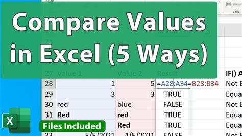
Finding missing values between two columns in Excel can be a common task, especially when working with large datasets. This process helps in identifying discrepancies, updating records, and ensuring data consistency across different lists or tables. Excel offers several methods to compare two columns and find missing values, ranging from using formulas to leveraging Excel's built-in features and add-ins. Here, we'll explore some of the most effective and efficient ways to accomplish this task.
When comparing two columns to find missing values, the goal is often to identify which entries are present in one column but not in the other. This can be done to synchronize two lists, find unique entries, or simply to audit and correct data discrepancies.
Understanding the Task
Before diving into the methods, it's essential to understand the nature of your data and what you're trying to achieve. Are you looking to find values that are in Column A but not in Column B, or vice versa, or perhaps both? Knowing this will guide your approach.
Method 1: Using Conditional Formatting
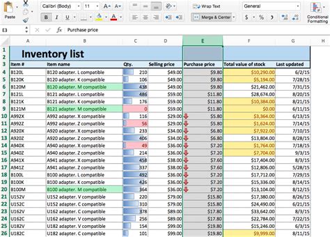
Conditional formatting can visually highlight cells that are unique to one column compared to another. While it doesn't directly tell you which values are missing, it can give you a quick visual cue.
- Select the range of cells in one of the columns.
- Go to the "Home" tab, find the "Styles" group, and click on "Conditional Formatting."
- Choose "New Rule," then select "Use a formula to determine which cells to format."
- Enter a formula like
=COUNTIF(B:B, A1)=0if you're selecting Column A and comparing it to Column B. This formula checks if the value in cell A1 appears anywhere in Column B. - Click "Format," choose how you want the cells to be highlighted, and click "OK."
Method 2: Using VLOOKUP
The VLOOKUP function can be used to find missing values by returning a value if it exists in another column and an error if it doesn't.
- Assume your data is in Columns A and B.
- In a new column (say, Column C), enter the formula
=VLOOKUP(A2, B:B, 1, FALSE). - If the value in A2 is found in Column B, it will return the value; otherwise, it will return a #N/A error.
- To highlight missing values, you can wrap the VLOOKUP in an IFERROR function, like
=IFERROR(VLOOKUP(A2, B:B, 1, FALSE), "Missing").
Method 3: Using INDEX/MATCH
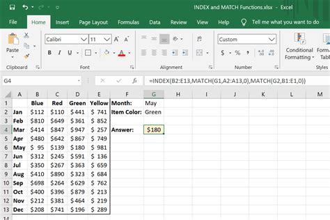
Similar to VLOOKUP but more flexible, the INDEX/MATCH function combination can also be used to find missing values.
- Use the formula
=INDEX(B:B, MATCH(A2, B:B, 0)). - If A2 is not found in Column B, this will return a #N/A error.
- Again, you can use IFERROR to return a custom message instead of the error, like
=IFERROR(INDEX(B:B, MATCH(A2, B:B, 0)), "Missing").
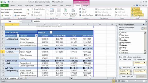
Method 4: Using PivotTables
PivotTables can be a powerful tool for comparing data and finding missing values, especially when dealing with large datasets.
- Select your data range (including headers).
- Go to the "Insert" tab and click on "PivotTable."
- Choose a cell to place your PivotTable and click "OK."
- Drag one column's header to the "Row Labels" area and the other to the "Row Labels" area as well, but below the first one.
- Right-click on the "Row Labels" dropdown and select "Filter" > "Select Multiple Items" to deselect any values you don't want to see.
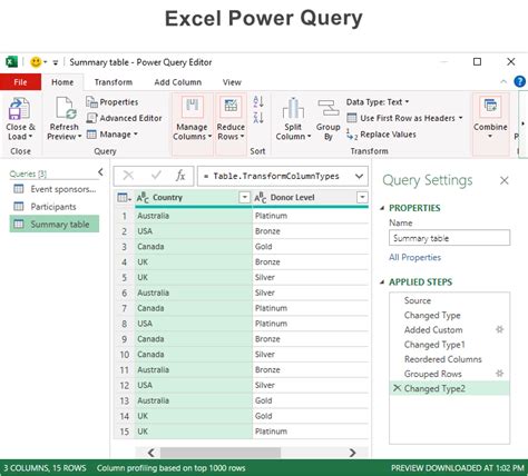
Method 5: Using Power Query
For more advanced users, Power Query (available in Excel 2010 and later versions) offers a robust way to compare and manipulate data.
- Select your data range and go to the "Data" tab.
- Click on "From Table/Range" to load your data into Power Query.
- Use the "Merge Queries" feature to compare your two columns, selecting "Merge as New" and choosing an outer join type that suits your needs (e.g., left outer to see values in Column A not in Column B).
Method 6: Using Formulas to Highlight Unique Values
You can use formulas directly in conditional formatting or in a separate column to highlight unique values.
- For values in A that are not in B:
=COUNTIF(B:B, A1)=0 - For values in B that are not in A:
=COUNTIF(A:A, B1)=0
Gallery of Excel Compare Features
Excel Compare Image Gallery


FAQs
What is the easiest way to compare two columns in Excel?
+The easiest way often involves using conditional formatting or a simple VLOOKUP function, depending on your specific needs and the size of your dataset.
How do I find missing values between two lists in Excel?
+You can use formulas like VLOOKUP or INDEX/MATCH, or utilize features like PivotTables and Power Query for more advanced comparisons.
Can I automate the process of comparing two columns in Excel?
+Yes, you can automate this process using macros or by leveraging Power Query for more complex data manipulations and comparisons.
In conclusion, comparing two columns to find missing values in Excel is a versatile task that can be approached from multiple angles, depending on the specifics of your data and what you aim to achieve. Whether you're looking for a quick visual comparison or a detailed, automated process, Excel's range of features and functions provides a solution tailored to your needs. By mastering these methods, you'll be better equipped to manage and analyze your data, ensuring accuracy, consistency, and efficiency in your work.
We invite you to share your experiences, tips, or questions regarding comparing columns in Excel in the comments below. Your insights can help others facing similar challenges, and together, we can explore the vast capabilities of Excel to enhance our productivity and data analysis skills.