5 Ways Excel Conditional Formatting

The importance of data analysis in today's fast-paced business world cannot be overstated. With the vast amounts of data being generated every day, it's crucial to have the right tools to make sense of it all. One such tool is Microsoft Excel, a powerful spreadsheet software that has been a staple in many industries for decades. Within Excel, there's a feature that stands out for its ability to enhance data visualization and analysis: Conditional Formatting. This feature allows users to highlight cells based on specific conditions, making it easier to identify trends, patterns, and outliers in their data. In this article, we'll delve into five ways Excel Conditional Formatting can be used to improve your data analysis.

Excel has been around for a long time, and over the years, it has evolved to include a wide range of features that cater to different needs. From basic calculations to complex data modeling, Excel is the go-to software for many professionals. However, with the increasing complexity of data, the need for better visualization tools has become more pressing. This is where Conditional Formatting comes in, providing a simple yet effective way to highlight important information in your spreadsheets. Whether you're a seasoned Excel user or just starting out, understanding how to use Conditional Formatting can significantly enhance your data analysis capabilities.

The applications of Conditional Formatting are diverse, ranging from identifying high and low values in a dataset to highlighting duplicate values or creating custom formatting rules based on formulas. This feature is not just about making your spreadsheets look more appealing; it's about uncovering insights that might be hidden in plain sight. By applying different formatting options such as colors, icons, and data bars, you can visually distinguish between different types of data, making it easier to understand and act upon the information. In the following sections, we'll explore five practical ways to use Excel Conditional Formatting to improve your data analysis and presentation.

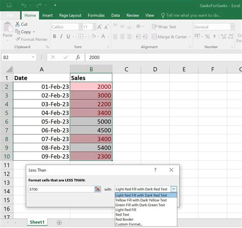
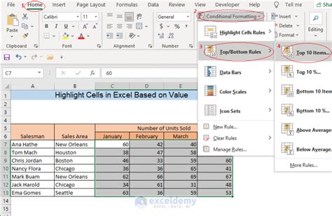
Highlighting Cells Based on Values

One of the most common uses of Conditional Formatting is to highlight cells based on their values. This can be particularly useful in identifying high or low performers in a dataset. For instance, if you have a list of sales figures, you might want to highlight any figure that exceeds a certain threshold. Excel makes this process straightforward by allowing you to apply formatting rules based on cell values, formulas, or even formatting icons. To highlight cells based on values, you simply need to select the range of cells you're interested in, go to the Home tab in Excel, click on Conditional Formatting, and then choose the type of rule you want to apply.

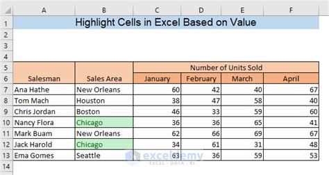
Steps to Highlight Cells Based on Values

To get started, follow these steps: - Select the cell or range of cells you want to format. - On the Home tab, click Conditional Formatting. - Choose "Highlight Cells Rules" and then select "Greater Than" or "Less Than" depending on your needs. - Enter the value you want to use as a threshold. - Click OK to apply the formatting.

Using Data Bars to Visualize Data

Data bars are another powerful tool within Conditional Formatting that can help in visualizing data trends. By representing data values as bars within cells, you can quickly see the relative size of each value. This is especially useful in comparing different data points across a range. For example, if you're analyzing website traffic over several months, data bars can give you a visual representation of how traffic has fluctuated, making it easier to identify peaks and troughs. To apply data bars, select your data range, go to Conditional Formatting, and choose "Data Bars" from the options.

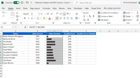
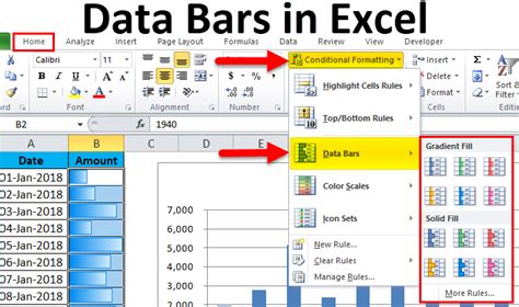
Benefits of Data Bars

The benefits of using data bars include: - Enhanced visualization: Data bars provide a quick and easy way to visualize data trends. - Easy comparison: They allow for easy comparison between different data points. - Customization: You can customize the appearance of data bars to suit your needs.

Highlighting Duplicate Values

Duplicate values can be a significant issue in data analysis, potentially leading to incorrect conclusions or skewed results. Conditional Formatting offers a simple way to identify these duplicates. By highlighting duplicate values, you can quickly spot and address any issues. This feature is particularly useful when working with large datasets where manual inspection might be impractical. To highlight duplicates, select your data range, go to Conditional Formatting, select "Highlight Cells Rules," and then choose "Duplicate Values."

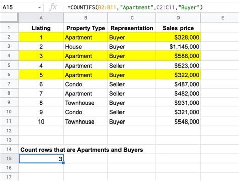
Why Identify Duplicate Values?

Identifying duplicate values is crucial because: - It helps in data cleaning: Duplicate values can affect the accuracy of your analysis. - It saves time: Automatically highlighting duplicates saves time compared to manual checking. - It improves data integrity: By removing duplicates, you ensure your data is more reliable.

Using Icon Sets

Icon sets are a visually appealing way to categorize and highlight data based on specific conditions. These icons can represent different states or values, such as trends, ratings, or statuses, making it easier to understand complex data at a glance. For example, in a customer satisfaction survey, you could use icon sets to represent different levels of satisfaction (e.g., happy face for satisfied, neutral face for average, and sad face for dissatisfied). To apply icon sets, select your data, go to Conditional Formatting, and choose "Icon Sets."

Advantages of Icon Sets

The advantages of using icon sets include: - Enhanced visualization: Icons can make data more engaging and easier to understand. - Customization: You can choose from a variety of icon sets to match your data and presentation style. - Flexibility: Icon sets can be applied to different types of data, from numerical values to text.

Creating Custom Rules with Formulas

For more advanced users, Conditional Formatting also offers the option to create custom rules using formulas. This feature provides unparalleled flexibility, allowing you to highlight cells based on virtually any condition you can think of. Whether it's highlighting dates that fall within a certain range, identifying text that contains specific keywords, or applying formatting based on the values in other cells, custom formulas can help. To create a custom rule, select your data range, go to Conditional Formatting, choose "New Rule," and then select "Use a formula to determine which cells to format."

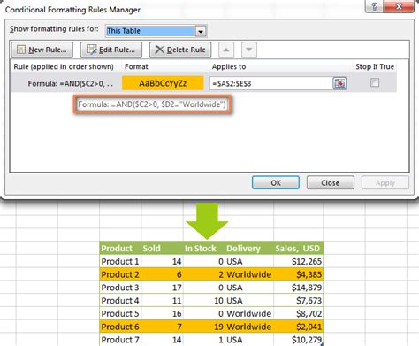
Applications of Custom Rules

Custom rules can be applied in various scenarios, such as: - Complex data analysis: Where standard formatting rules are not enough. - Specific conditions: That require unique formulas to identify. - Integration with other Excel functions: To create dynamic and interactive spreadsheets.

Excel Conditional Formatting Image Gallery

What is Conditional Formatting in Excel?

+

Conditional Formatting is a feature in Excel that allows you to highlight cells based on specific conditions, making it easier to identify trends, patterns, and outliers in your data.

How do I apply Conditional Formatting in Excel?

+

To apply Conditional Formatting, select the cell or range of cells you want to format, go to the Home tab, click on Conditional Formatting, and then choose the type of rule you want to apply.

What are the benefits of using Conditional Formatting?

+

The benefits include enhanced data visualization, easy identification of trends and patterns, and improved data analysis capabilities.

Can I create custom Conditional Formatting rules?

+

How do I highlight duplicate values using Conditional Formatting?

+

To highlight duplicates, select your data range, go to Conditional Formatting, select "Highlight Cells Rules," and then choose "Duplicate Values."

In conclusion, Excel Conditional Formatting is a powerful tool that can significantly enhance your data analysis and presentation capabilities. By understanding how to apply different types of formatting rules, from highlighting cells based on values to creating custom rules with formulas, you can uncover insights in your data that might otherwise remain hidden. Whether you're a beginner or an advanced Excel user, mastering Conditional Formatting can take your data analysis to the next level. We invite you to share your experiences with Conditional Formatting, ask questions, or explore more advanced techniques in the comments section below. Don't forget to share this article with colleagues or friends who might benefit from learning more about this versatile feature in Excel.