Highlight Row If Cell Contains In Excel

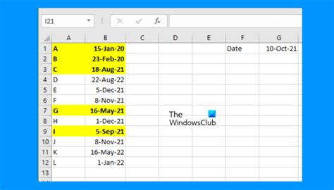
Highlighting rows in Excel based on specific cell contents can significantly enhance data analysis and visualization. This feature allows users to quickly identify important information, trends, or anomalies within their datasets. Excel provides several methods to achieve this, including using Conditional Formatting, a powerful tool that enables users to apply formatting to a cell or range of cells based on specific conditions.

The importance of highlighting rows cannot be overstated, especially in large datasets where manual scanning for specific data points can be time-consuming and prone to errors. By applying conditional formatting, users can automate the process of highlighting cells that meet certain criteria, such as containing specific text, numbers, or dates. This not only saves time but also improves the readability and usability of the spreadsheet.

For individuals and organizations dealing with vast amounts of data, being able to highlight rows based on cell contents is crucial for data-driven decision-making. It helps in identifying patterns, outliers, and critical data points that might require immediate attention. Moreover, the ability to customize the formatting options (e.g., fill color, font color, borders) allows users to tailor the visualization to their specific needs or preferences.

In addition to its practical applications, highlighting rows in Excel is also a testament to the software's flexibility and adaptability. Whether you're a beginner looking to organize personal finances or a professional analyzing complex market trends, Excel's conditional formatting feature is an indispensable tool. Its ease of use, combined with its powerful capabilities, makes it an essential skill for anyone working with data.

How to Highlight Rows in Excel

To highlight rows in Excel based on cell contents, follow these steps:

1. Select the Range: First, select the entire range of cells that you want to format, including headers.
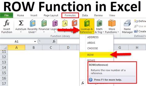
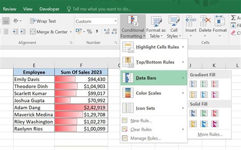
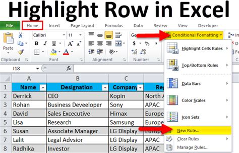
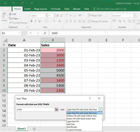
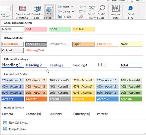
2. Go to Conditional Formatting: Navigate to the "Home" tab on the Excel ribbon, find the "Styles" group, and click on "Conditional Formatting."
3. New Rule: In the Conditional Formatting dropdown menu, select "New Rule." This opens the New Formatting Rule dialog box.
4. Use a Formula: Choose "Use a formula to determine which cells to format." This option allows you to specify a condition based on a formula.
5. Enter the Formula: In the formula box, you can enter a formula that identifies the condition under which a row should be highlighted. For example, to highlight rows where the cell in column A contains the word "example," you could use a formula like =ISNUMBER(SEARCH("example",A1)), assuming A1 is the first cell in your selected range that you want to check.
6. Format: Click on the "Format" button to choose how you want the highlighted rows to appear (e.g., fill color, font).
7. Apply: Click "OK" to apply the rule. Excel will then highlight the rows based on your specified condition.

Common Formulas for Highlighting Rows

Several formulas can be used to highlight rows based on different conditions:

• Exact Match: To highlight rows where a cell exactly matches a specific text, you can use =A1="exact text".
• Contains: For cells that contain specific text anywhere within the cell, use =ISNUMBER(SEARCH("text",A1)).
• Starts With: To highlight rows where the cell starts with specific text, use =LEFT(A1,LEN("text"))="text".
• Ends With: For rows where the cell ends with specific text, the formula is =RIGHT(A1,LEN("text"))="text".

Multiple Conditions

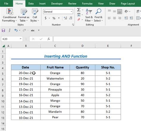
Sometimes, you may need to highlight rows based on multiple conditions. Excel's conditional formatting allows for this through the use of the AND and OR functions within your formulas:

• AND: To highlight rows where two conditions are met, use =AND(condition1, condition2).
• OR: For rows where at least one of two conditions is met, use =OR(condition1, condition2).

Highlighting Rows with Multiple Criteria

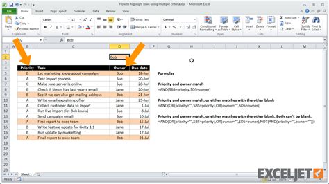
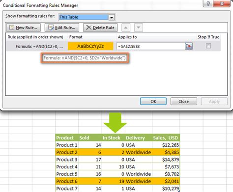
When dealing with more complex datasets, you might need to apply formatting based on multiple criteria across different columns. This can be achieved by combining the AND or OR functions with the conditional formatting rules.

For instance, to highlight rows where column A contains "example" and column B is greater than 10, you could use the formula =AND(ISNUMBER(SEARCH("example",A1)),B1>10).

Managing and Editing Conditional Formatting Rules

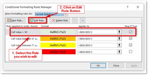
After applying conditional formatting rules, you may need to manage or edit them, especially if your data changes or if you want to apply different conditions. Excel allows you to easily view, edit, and delete existing rules:

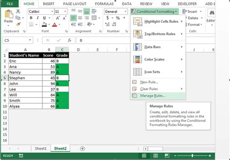
1. Go to the "Home" tab and click on "Conditional Formatting."
2. Select "Manage Rules" to open the Conditional Formatting Rules Manager dialog box.
3. Here, you can add new rules, edit existing ones, or delete rules that are no longer needed.

Best Practices for Using Conditional Formatting

To get the most out of conditional formatting and to keep your spreadsheets organized and efficient:

• Keep it Simple: Start with simple rules and gradually move to more complex conditions as needed.
• Use Clear Formulas: Ensure your formulas are easy to understand and maintain.
• Test Thoroughly: Always test your rules with sample data to ensure they work as expected.
• Document Your Work: Especially in shared spreadsheets, consider documenting the rules and formulas used for clarity and future reference.

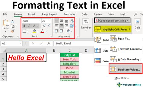
Gallery of Excel Formatting Examples

Excel Formatting Image Gallery

How do I highlight rows in Excel based on cell contents?

+

To highlight rows in Excel based on cell contents, use the Conditional Formatting feature. Select the range, go to Home > Conditional Formatting, choose New Rule, and then use a formula to determine which cells to format.

What formulas can I use to highlight rows based on specific conditions?

+

You can use various formulas such as exact match, contains, starts with, and ends with. For example, to highlight rows where a cell contains "example," you can use the formula =ISNUMBER(SEARCH("example",A1)).

How do I manage and edit conditional formatting rules in Excel?

+

To manage and edit conditional formatting rules, go to Home > Conditional Formatting > Manage Rules. Here, you can add new rules, edit existing ones, or delete rules that are no longer needed.

In conclusion, highlighting rows in Excel based on cell contents is a powerful feature that enhances data analysis and visualization. By mastering conditional formatting and understanding how to apply different formulas and rules, users can unlock the full potential of Excel for their data management needs. Whether you're working with simple datasets or complex spreadsheets, the ability to highlight important information can significantly improve your productivity and decision-making capabilities. Feel free to share your experiences or ask questions about using conditional formatting in Excel in the comments below.