Intro
The combination of INDEX and MATCH functions in Excel VBA is a powerful tool for looking up and retrieving data from tables and ranges. It offers more flexibility and is often more efficient than the traditional VLOOKUP function. For those who are familiar with Excel and are looking to enhance their skills in using VBA (Visual Basic for Applications), mastering the INDEX-MATCH function combination is essential. Here are five Excel VBA INDEX-MATCH tips to help you become more proficient in data manipulation and analysis.
When working with data in Excel, being able to quickly and accurately retrieve specific information is crucial. The INDEX-MATCH function combination is particularly useful because it allows for lookups in any column of a table, not just the first column as with VLOOKUP. Moreover, it is less prone to errors when the structure of the table changes. Understanding how to effectively use INDEX-MATCH in VBA can significantly streamline your workflow and improve your productivity.
One of the key benefits of using INDEX-MATCH is its ability to perform lookups without the limitations imposed by other functions. It can handle large datasets efficiently and is less likely to cause errors due to column insertions or deletions. However, to fully leverage the potential of INDEX-MATCH in VBA, it's essential to grasp the basics of how these functions work together and how they can be applied in various scenarios.
Understanding INDEX and MATCH Functions
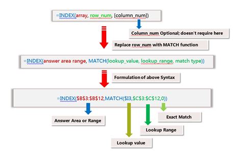
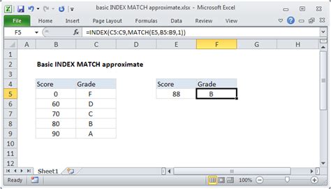
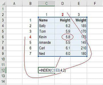
Before diving into the tips, let's briefly cover the basics of the INDEX and MATCH functions. The INDEX function returns a value or the reference to a value from a given range. The MATCH function returns the position of a value within a range. When used together, they form a powerful lookup combination. The syntax for the INDEX-MATCH function combination is INDEX(range, MATCH(lookup_value, lookup_array, [match_type]), where range is the range from which to return a value, lookup_value is the value you want to look up, lookup_array is the range where you want to look up the value, and match_type specifies whether you want an exact match or an approximate match.
Tip 1: Basic INDEX-MATCH Lookup
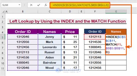
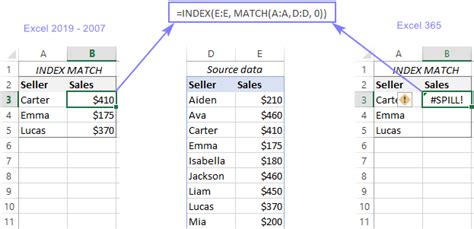
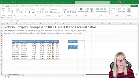
The first tip is to understand how to perform a basic lookup using INDEX-MATCH. This involves specifying the range from which you want to retrieve data, the value you're looking for, and the array where this value is located. For example, if you have a table with employee names in column A and their corresponding IDs in column B, and you want to find the ID of a specific employee, you can use the INDEX-MATCH function combination.Performing Lookups with INDEX-MATCH
To perform this lookup, you would use a formula like =INDEX(B:B, MATCH("EmployeeName", A:A, 0)), where B:B is the range with the IDs, "EmployeeName" is the name of the employee you're looking for, A:A is the range with the employee names, and 0 specifies that you want an exact match.
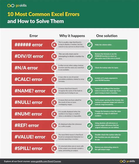
Tip 2: Handling Errors with IFERROR
The second tip involves handling errors that might occur when the lookup value is not found. The IFERROR function can be used to return a custom value instead of the `#N/A` error that Excel typically displays when it cannot find a match. This is particularly useful for cleaning up your data and making your spreadsheets more user-friendly.Error Handling in INDEX-MATCH
For example, you could modify the previous formula to =IFERROR(INDEX(B:B, MATCH("EmployeeName", A:A, 0)), "Employee not found"). This way, if the employee name is not found in the list, the formula will return the message "Employee not found" instead of an error.
Tip 3: Using INDEX-MATCH with Multiple Criteria
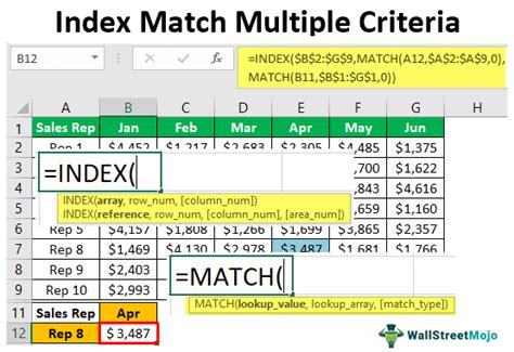
The third tip is about using INDEX-MATCH with multiple criteria. This can be achieved by using the MATCH function in combination with the INDEX function in an array formula. You create an array of relative positions of the rows that match both criteria and then use the INDEX function to return the value at the first position in that array.Multiple Criteria Lookups
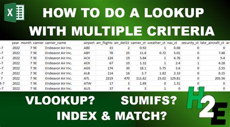
For instance, if you want to find the ID of an employee based on both the first and last name, you could use an array formula like =INDEX(B:B, MATCH(1, (A:A="FirstName") * (C:C="LastName"), 0)), assuming the first names are in column A and the last names are in column C.
Tip 4: Dynamic Range Adjustment
The fourth tip involves adjusting the range dynamically based on the data. This can be particularly useful when your dataset is constantly changing. By using the OFFSET function in combination with the COUNTA function, you can create a dynamic range that automatically adjusts as your data grows or shrinks.Dynamic Range in INDEX-MATCH
For example, if your data starts in cell A1 and you want the range to automatically include all cells with data in column A, you could use =INDEX(OFFSET(A1, 0, 0, COUNTA(A:A), 1), MATCH("EmployeeName", OFFSET(A1, 0, 0, COUNTA(A:A), 1), 0)). This formula adjusts the range based on the number of cells with data in column A.
Tip 5: Applying INDEX-MATCH in VBA
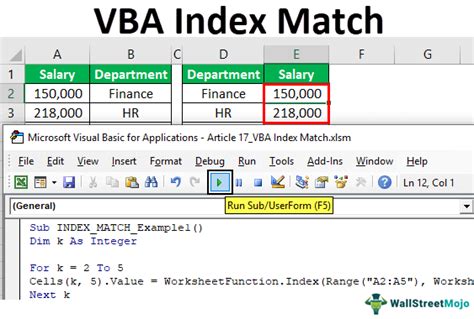
The fifth tip is about applying the INDEX-MATCH function combination in VBA. While the formulas can be powerful in Excel sheets, using them in VBA scripts can offer even more flexibility and automation capabilities. You can use VBA to loop through data, perform lookups, and update values dynamically.INDEX-MATCH in VBA

To apply INDEX-MATCH in a VBA script, you would first define your ranges and lookup values as variables, then use these variables within your VBA code to perform the lookup and retrieve the desired value. For example, you might use Dim lookupRange As Range, Set lookupRange = Range("A1:A100"), and then result = Application.Index(Range("B1:B100"), Application.Match("EmployeeName", lookupRange, 0)).
INDEX-MATCH Function Gallery


What is the INDEX-MATCH function combination used for?
+The INDEX-MATCH function combination is used for looking up and retrieving data from tables and ranges in Excel. It offers more flexibility and is often more efficient than the traditional VLOOKUP function.
How does the INDEX function work in Excel?
+The INDEX function returns a value or the reference to a value from a given range. It is often used in combination with the MATCH function to perform lookups.
What is the purpose of the MATCH function in the INDEX-MATCH combination?
+The MATCH function returns the position of a value within a range. When used with the INDEX function, it helps to locate the value to be retrieved.
Can the INDEX-MATCH function combination handle multiple criteria lookups?
+Yes, the INDEX-MATCH function combination can handle multiple criteria lookups by using array formulas that create an array of relative positions of the rows that match all the criteria.
How can I apply the INDEX-MATCH function combination in VBA?
+You can apply the INDEX-MATCH function combination in VBA by defining your ranges and lookup values as variables and then using these variables within your VBA code to perform the lookup and retrieve the desired value.
In conclusion, mastering the INDEX-MATCH function combination is a valuable skill for anyone working with data in Excel. Whether you're performing simple lookups or complex data analysis, understanding how to effectively use these functions can significantly enhance your productivity and the accuracy of your work. By applying the tips outlined above and practicing with different scenarios, you can become proficient in using INDEX-MATCH to streamline your workflow and improve your data management capabilities. We invite you to share your experiences and tips on using the INDEX-MATCH function combination in the comments below and to explore more articles on Excel functions and VBA programming to further expand your skills.