Google Sheets Sum Column If Another Column

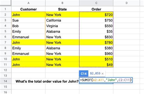
The ability to sum a column in Google Sheets based on the values in another column is a powerful feature that allows for dynamic and conditional calculations. This can be particularly useful for data analysis, financial calculations, and tracking inventory or sales performance based on specific criteria. The most common way to achieve this is by using the SUMIF or SUMIFS functions, which are part of Google Sheets' repertoire of functions.

To start, let's consider a basic scenario where you have a list of items, their categories, and their respective costs. You want to sum up the costs of items that belong to a specific category. Here's how you can do it:

Using SUMIF

The SUMIF function in Google Sheets is used to sum up a range of cells based on a condition that you specify. The syntax for SUMIF is as follows:

SUMIF(range, criterion, [sum_range])

• range is the range of cells that you want to apply the condition to.
• criterion is the condition that must be met for a cell to be included in the sum.
• [sum_range] is optional and specifies the actual cells to sum. If omitted, Google Sheets sums the values in the range specified.

Let's say you have the following data:

• Column A contains the categories of items.
• Column B contains the costs of the items.

You want to sum the costs of all items in the category "Electronics". Your data looks like this:

Category	Cost
Electronics	100
Toys	50
Electronics	200
Books	20
Electronics	150

Assuming your data is in the range A1:B5, you can use the SUMIF function like this:

=SUMIF(A1:A5, "Electronics", B1:B5)

This formula sums up the costs in column B for all rows where the category in column A is "Electronics".

Using SUMIFS

If you need to apply multiple conditions, you can use the SUMIFS function. The syntax for SUMIFS is:

SUMIFS(sum_range, criteria_range1, criterion1, [criteria_range2], [criterion2],...)

• sum_range is the range of cells to sum.
• criteria_range1 is the range of cells to apply the first condition.
• criterion1 is the first condition.
• You can add more criteria_range and criterion pairs as needed.

Let's say you now have an additional column, Column C, for the item's subcategory, and you want to sum the costs of items that are in the category "Electronics" and subcategory "Smartphones". Your data might look like this:

Category	Subcategory	Cost
Electronics	Smartphones	100
Toys	Dolls	50
Electronics	Smartphones	200
Books	Novels	20
Electronics	Laptops	150

You can use SUMIFS like this:

=SUMIFS(B1:B5, A1:A5, "Electronics", C1:C5, "Smartphones")

This formula sums the costs in column B for all rows where the category is "Electronics" and the subcategory is "Smartphones".

Practical Examples and Applications

These functions are incredibly versatile and can be applied to a wide range of scenarios, including but not limited to:

• Financial Analysis: Summing revenues or expenses based on departments, regions, or product lines.
• Inventory Management: Calculating the total value of stock based on categories, suppliers, or storage locations.
• Sales Performance: Summing sales amounts based on sales regions, product categories, or sales teams.

Tips for Effective Use

• Use Absolute References: When copying formulas down or across, consider using absolute references ($A$1) for the range and criterion parts of the formula to ensure they don't change.
• Named Ranges: For complex or large datasets, consider defining named ranges for your criteria ranges and sum ranges to make the formulas more readable.
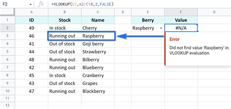
• Error Handling: Be aware that if the criterion is not found, SUMIF and SUMIFS return 0. If you expect the criterion to always be present, this is fine, but in other cases, you might want to add error handling to highlight missing criteria.

Advanced Scenarios

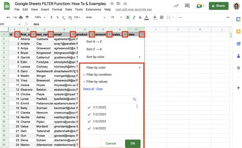
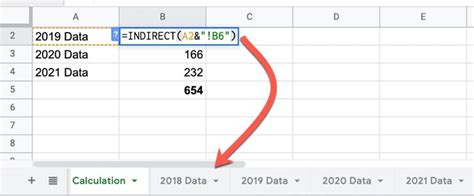
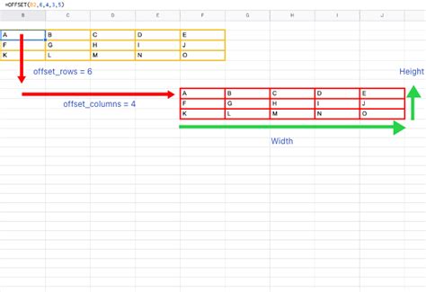
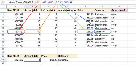
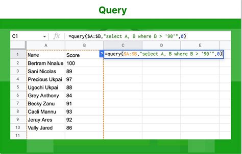
For more complex scenarios, such as summing based on multiple conditions across different sheets or using dynamic criteria, you might need to combine SUMIF or SUMIFS with other Google Sheets functions, such as INDIRECT, OFFSET, or INDEX/MATCH. The use of arrays and the FILTER function can also provide powerful alternatives for summing based on conditions.

Gallery of Google Sheets Functions

Google Sheets Functions Gallery

FAQs

What is the main difference between SUMIF and SUMIFS?

+

SUMIF is used for a single condition, while SUMIFS allows for multiple conditions to be applied.

Can I use SUMIF or SUMIFS with dates as criteria?

+

Yes, you can use dates as criteria in SUMIF and SUMIFS. However, ensure your dates are in a format that Google Sheets recognizes as dates.

How do I handle errors when using SUMIF or SUMIFS?

+

Use error handling functions like IFERROR or IFNA to manage errors, such as when the criterion is not found.

In conclusion, mastering the use of SUMIF and SUMIFS in Google Sheets can significantly enhance your data analysis capabilities. Whether you're working with simple or complex datasets, these functions provide a powerful tool for conditional summing. By combining them with other Google Sheets functions and features, you can unlock even more advanced data manipulation and analysis capabilities. We invite you to share your experiences or ask further questions about using these functions in the comments below.