Intro
Master listing in Excel with 5 easy methods, including sorting, filtering, and formatting data, to create organized lists and tables, enhancing data analysis and visualization with Excel formulas and functions.
When working with data in Excel, listing and organizing information is crucial for efficient analysis and presentation. Excel offers various methods to create and manage lists, each with its own set of benefits and applications. Understanding these methods can significantly enhance your productivity and the clarity of your spreadsheets. In this article, we will delve into five ways to list in Excel, exploring their uses, step-by-step guides on how to implement them, and tips for maximizing their potential.
The ability to effectively list data is fundamental in Excel, as it allows users to categorize, analyze, and present information in a structured and understandable format. Whether you are managing inventory, tracking sales, or organizing project tasks, Excel's listing capabilities are indispensable. Moreover, with the constant evolution of Excel, incorporating new features and functions, staying updated on the best practices for listing data is essential for any user looking to leverage the full potential of this powerful tool.
Excel's versatility in handling and manipulating data makes it an indispensable tool for both personal and professional use. From simple to-do lists to complex databases, Excel can accommodate a wide range of data management needs. The key to unlocking its full potential lies in understanding the various techniques available for creating, editing, and analyzing lists. By mastering these techniques, users can streamline their workflow, enhance data visualization, and make more informed decisions based on their data.
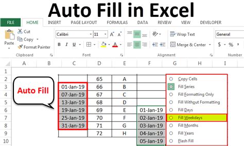
1. Using AutoFill to Create Lists
One of the quickest and most efficient ways to create lists in Excel is by using the AutoFill feature. This feature allows users to automatically fill a range of cells with a series of numbers, dates, or text based on the pattern established in the initial cells. To use AutoFill, select the cells containing the initial data, move your cursor to the bottom-right corner of the selection until it changes into a cross, and then drag it down or across to fill the desired range.
For example, if you need a list of numbers from 1 to 100, you can simply type "1" and "2" in the first two cells, select both cells, and then use AutoFill to generate the rest of the list. Similarly, for a list of dates, you can enter the first date and use AutoFill to continue the sequence. This feature is not only time-saving but also reduces the likelihood of errors that can occur with manual entry.
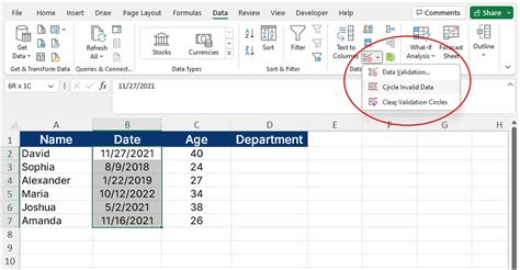
2. Creating Drop-Down Lists with Data Validation

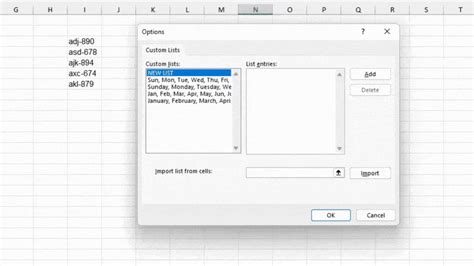
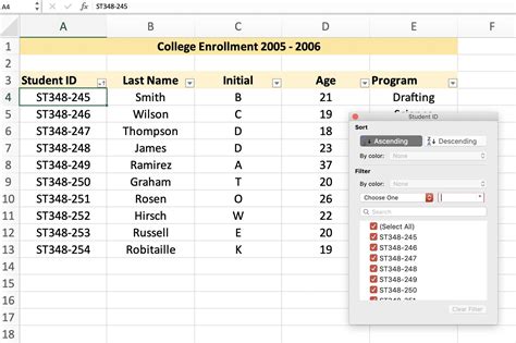
Drop-down lists are incredibly useful for restricting input to a specific set of options, thereby ensuring data consistency and reducing errors. To create a drop-down list in Excel, you can use the Data Validation feature. First, select the cell where you want the drop-down list to appear. Then, go to the "Data" tab on the ribbon, click on "Data Validation," and select "Settings." In the "Allow" field, choose "List" and specify the range of cells containing the list of options or directly enter the list using a comma to separate each item.
For instance, if you're creating a spreadsheet for order tracking and you want to limit the "Status" field to "Pending," "Shipped," or "Delivered," you can create a drop-down list with these options. This not only helps in maintaining uniformity in data entry but also makes it easier to filter or analyze the data based on these categories.
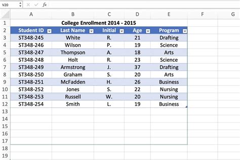
3. Using Tables to Organize Lists
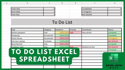
Excel tables are a powerful tool for organizing and managing lists. They offer features like automatic filtering, sorting, and formatting, making it easier to analyze and present data. To create a table, select the range of cells containing your list, go to the "Insert" tab, and click on "Table." You can then customize your table by adding headers, applying styles, and using the filter buttons to narrow down your data.
Tables are particularly useful for lists that require frequent updates or need to be shared with others. The structured format of a table enhances readability and facilitates collaboration. Moreover, Excel tables can be easily converted into pivot tables for more advanced data analysis, allowing users to summarize, analyze, and visualize large datasets.
4. Creating Lists with PivotTables
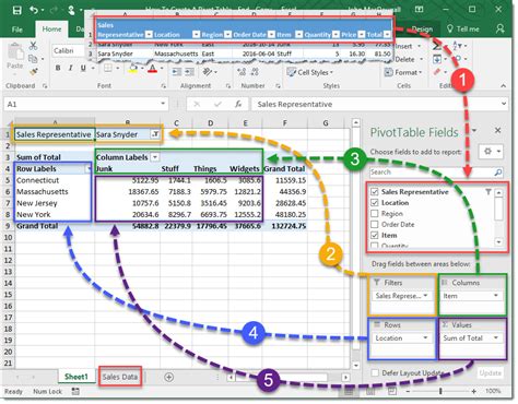
PivotTables are a dynamic way to create lists that summarize large datasets. They enable users to rotate and aggregate data fields, creating custom lists that highlight specific trends or patterns. To create a PivotTable, select a cell where you want the PivotTable to be placed, go to the "Insert" tab, and click on "PivotTable." Then, choose the table or range of cells you want to analyze and follow the prompts to set up your PivotTable.
PivotTables are invaluable for creating dynamic lists that can be easily updated or modified based on changes in the underlying data. For example, if you have a dataset of sales figures by region and product, you can use a PivotTable to create a list of the top-selling products in each region, which can be instantly updated if new sales data becomes available.
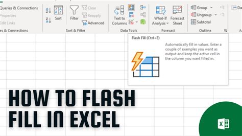
5. Using Flash Fill to Extract and Create Lists
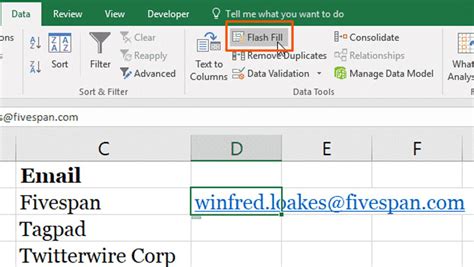
Flash Fill is a feature in Excel that can automatically extract and create lists based on patterns it detects in your data. This feature is particularly useful for splitting or combining data into separate columns. To use Flash Fill, simply type the first few entries of the list you want to create in the desired format, select those cells, and then go to the "Data" tab and click on "Flash Fill" or press "Ctrl + E."
For instance, if you have a list of full names in one column and you want to create separate columns for first and last names, Flash Fill can automatically populate these columns based on the pattern you establish in the first few cells. This feature saves time and reduces the effort required to manipulate and organize data, making it a valuable tool for anyone working with lists in Excel.
Excel List Creation Image Gallery


What is the best way to create a list in Excel for data analysis?
+The best way to create a list in Excel for data analysis depends on the nature of the data and the analysis requirements. However, using tables and pivot tables can provide a structured and dynamic approach to data analysis.
How do I automatically update a list in Excel when new data is added?
+You can automatically update a list in Excel by using dynamic ranges or tables. These features allow the list to expand or contract based on the addition or removal of data.
What is the difference between a regular list and a table in Excel?
+A regular list in Excel is a simple range of cells containing data, whereas a table is a structured range with enhanced features like filtering, sorting, and formatting. Tables also support dynamic updates and can be easily converted into pivot tables for advanced analysis.
In conclusion, mastering the art of listing in Excel is a fundamental skill that can significantly enhance your productivity and data analysis capabilities. By understanding and leveraging the various methods available, from AutoFill and data validation to tables and pivot tables, you can create, manage, and analyze lists more efficiently. Whether you're a beginner or an advanced user, exploring these features and techniques will help you unlock the full potential of Excel and streamline your workflow. So, take the first step today, and discover how listing in Excel can transform the way you work with data. Share your thoughts on your favorite method for creating lists in Excel, and don't forget to share this article with anyone who could benefit from these powerful techniques.