5 Ways Reverse Excel Order

The ability to reverse the order of data in Excel can be incredibly useful for a variety of tasks, from organizing data for analysis to preparing it for presentation. Whether you're working with a small dataset or a large spreadsheet, knowing how to reverse the order of your data can save you a significant amount of time and effort. In this article, we'll explore five different ways to reverse the order of data in Excel, each with its own unique advantages and applications.

Reversing the order of data in Excel can be particularly useful when you need to analyze data from the most recent to the oldest, or when you want to highlight the most significant changes or trends in your data. By reversing the order of your data, you can quickly and easily identify patterns and insights that might be hidden when the data is presented in its original order. Additionally, reversing the order of data can be useful when preparing reports or presentations, as it allows you to highlight the most important or relevant information first.

One of the key benefits of reversing the order of data in Excel is that it can help to improve the clarity and readability of your data. By presenting data in a logical and intuitive order, you can make it easier for others to understand and analyze, which can be particularly useful when working with large or complex datasets. Furthermore, reversing the order of data can also help to reduce errors and inconsistencies, as it allows you to quickly and easily identify any discrepancies or anomalies in your data.

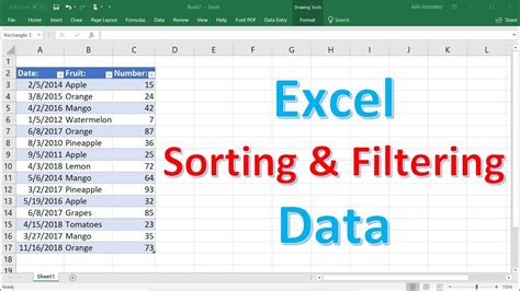
Method 1: Using the Sort & Filter Tool

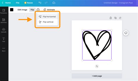
The Sort & Filter tool in Excel is one of the most straightforward ways to reverse the order of data. To use this tool, simply select the data range you want to reverse, go to the "Data" tab in the ribbon, and click on the "Sort & Filter" button. From here, you can select the column you want to sort by and choose the "Descending" or "Ascending" option to reverse the order of your data.

Method 2: Using the Flip Vertical Tool

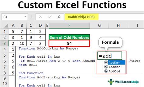
The Flip Vertical tool in Excel is another useful way to reverse the order of data. To use this tool, select the data range you want to reverse, go to the "Home" tab in the ribbon, and click on the "Find & Select" button. From here, select "Go To" and then "Special" to open the "Go To Special" dialog box. Select "Last cell" and then click "OK" to move to the last cell in your data range. Then, select the entire data range and go to the "Home" tab in the ribbon, click on the "Find & Select" button, and select "Flip Vertical" to reverse the order of your data.

Method 3: Using a Formula

Using a formula to reverse the order of data in Excel can be a powerful and flexible way to manipulate your data. One common formula used to reverse the order of data is the INDEX and MATCH functions. To use this formula, enter the following formula in a new column: `=INDEX(range,MATCH(ROW(range),ROW(range),0))`, where "range" is the data range you want to reverse. This formula will return the values in your data range in reverse order.

Method 4: Using VBA Macro

Using a VBA macro to reverse the order of data in Excel can be a useful way to automate repetitive tasks and improve productivity. To use a VBA macro, open the Visual Basic Editor by pressing "Alt + F11" or by navigating to the "Developer" tab in the ribbon and clicking on the "Visual Basic" button. Then, create a new module by clicking "Insert" and "Module" and enter the following code: `Sub ReverseData()`, `Range("A1:A10").Select`, `Selection.Reverse`, `End Sub`, where "A1:A10" is the data range you want to reverse. Finally, click "Run" to execute the macro and reverse the order of your data.

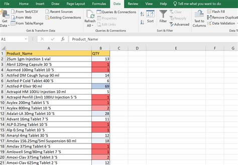
Method 5: Using Power Query

Using Power Query to reverse the order of data in Excel can be a powerful and flexible way to manipulate and analyze large datasets. To use Power Query, select the data range you want to reverse and go to the "Data" tab in the ribbon. Click on the "From Table/Range" button to open the Power Query Editor. Then, click on the "Add Column" tab and select "Index Column" to add a new column with a unique index for each row. Next, click on the "Home" tab and select "Sort & Filter" to sort the data by the index column in descending order. Finally, click on the "Load" button to load the reversed data into a new worksheet.

Gallery of Excel Order Reversal Methods

Excel Order Reversal Methods Image Gallery

What is the easiest way to reverse the order of data in Excel?

The easiest way to reverse the order of data in Excel is by using the Sort & Filter tool. Simply select the data range, go to the "Data" tab, and click on the "Sort & Filter" button. Then, select the column you want to sort by and choose the "Descending" or "Ascending" option to reverse the order of your data.

Can I use a formula to reverse the order of data in Excel?

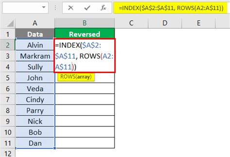
Yes, you can use a formula to reverse the order of data in Excel. One common formula used to reverse the order of data is the INDEX and MATCH functions. Simply enter the formula `=INDEX(range,MATCH(ROW(range),ROW(range),0))` in a new column, where "range" is the data range you want to reverse.

How do I reverse the order of data in Excel using VBA macro?

To reverse the order of data in Excel using VBA macro, open the Visual Basic Editor by pressing "Alt + F11" or by navigating to the "Developer" tab in the ribbon and clicking on the "Visual Basic" button. Then, create a new module and enter the code `Sub ReverseData()`, `Range("A1:A10").Select`, `Selection.Reverse`, `End Sub`, where "A1:A10" is the data range you want to reverse. Finally, click "Run" to execute the macro and reverse the order of your data.

What are the benefits of reversing the order of data in Excel?

The benefits of reversing the order of data in Excel include improving the clarity and readability of your data, reducing errors and inconsistencies, and highlighting the most important or relevant information first. Reversing the order of data can also help to identify patterns and insights that might be hidden when the data is presented in its original order.

Can I use Power Query to reverse the order of data in Excel?

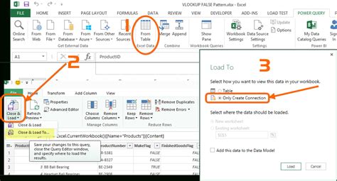
Yes, you can use Power Query to reverse the order of data in Excel. Simply select the data range, go to the "Data" tab, and click on the "From Table/Range" button to open the Power Query Editor. Then, click on the "Add Column" tab and select "Index Column" to add a new column with a unique index for each row. Next, click on the "Home" tab and select "Sort & Filter" to sort the data by the index column in descending order. Finally, click on the "Load" button to load the reversed data into a new worksheet.

In conclusion, reversing the order of data in Excel can be a useful and powerful tool for data analysis and presentation. By using one of the five methods outlined in this article, you can quickly and easily reverse the order of your data and improve the clarity and readability of your spreadsheets. Whether you're working with a small dataset or a large spreadsheet, knowing how to reverse the order of your data can save you a significant amount of time and effort. We encourage you to try out these methods and explore the many benefits of reversing the order of data in Excel. If you have any questions or need further assistance, please don't hesitate to comment or share this article with others.