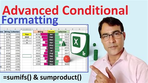
Excel Up Down Arrows Conditional Formatting

When working with data in Excel, it's often helpful to visualize trends and changes in values. One effective way to do this is by using conditional formatting to display up and down arrows based on the changes in values. This feature allows you to quickly identify increases and decreases in your data, making it easier to analyze and understand trends.

The importance of visualizing data trends cannot be overstated. By using up and down arrows, you can effortlessly scan through large datasets to pinpoint areas where values are increasing or decreasing. This can be particularly useful in financial analysis, where tracking changes in stock prices, sales figures, or other metrics is crucial. Moreover, in project management, identifying trends in task completion rates, resource allocation, or team performance can help in making informed decisions.

To apply this formatting, you first need to understand the basics of conditional formatting in Excel. Conditional formatting is a feature that allows you to apply different formats to cells based on specific conditions. You can use it to highlight cells that contain certain values, dates, or formulas. The process of applying up and down arrows involves creating a rule that compares cell values and then applies the appropriate arrow symbol based on whether the value has increased or decreased.

Setting Up Conditional Formatting for Up and Down Arrows

To set up conditional formatting for up and down arrows, follow these steps:

Select the range of cells that you want to format.
Go to the "Home" tab in the Excel ribbon and click on "Conditional Formatting."
Choose "New Rule" to create a custom formatting rule.
Select "Use a formula to determine which cells to format."
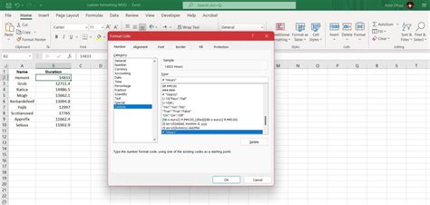
Enter a formula that compares the cell values. For example, to show an up arrow if the current value is greater than the previous one, you might use a formula like =A2>A1, assuming the values are in column A.
Click "Format" and choose a format that includes an up arrow. You can use the "Wingdings" font to find arrow symbols.
Repeat the process for the down arrow, using a formula like =A2<A1 and choosing a format with a down arrow.

Using Formulas for Dynamic Comparison

When setting up the formulas for comparing cell values, it's essential to consider the structure of your data. If your data is in a column, comparing each cell to the one above or below it is straightforward. However, if your data is structured differently, you may need to adjust your formulas accordingly. Using relative and absolute references can help you create formulas that work across your entire dataset.

Applying Up and Down Arrows with Icons

Another way to apply up and down arrows is by using the "Icon Sets" feature within conditional formatting. This method is more straightforward and doesn't require you to manually select fonts or create custom formulas for each condition.

Select your cell range.
Go to "Conditional Formatting" and choose "Icon Sets."
Select the icon set that includes up and down arrows.
Adjust the criteria for each icon by clicking on "Edit Rule."
Choose the type of comparison you want to make (e.g., "Cell Value," "Formula") and set your criteria.

Benefits of Using Icon Sets

Using icon sets for up and down arrows offers several benefits. It's quicker and easier to set up compared to creating custom rules for each condition. Additionally, icon sets can be easily applied to large datasets, and they automatically adjust based on the criteria you set. This feature is particularly useful when you need to analyze data trends across multiple rows or columns.

Customizing Your Conditional Formatting

While Excel's built-in conditional formatting options are powerful, you may find situations where you need more customization. This could involve using different colors, symbols, or even creating complex rules that combine multiple conditions. To customize your conditional formatting further:

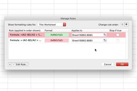
Use the "Manage Rules" option under "Conditional Formatting" to edit or delete existing rules.
Experiment with different formats and icons to find the combination that best represents your data.
Consider using VBA macros for highly customized or dynamic formatting needs.

Advanced Conditional Formatting Techniques

For more advanced users, Excel offers the capability to create complex conditional formatting rules using formulas and VBA. This can include applying formatting based on the values in other worksheets, using IF statements to combine conditions, or even creating interactive dashboards that update in real-time based on user input.

Best Practices for Using Up and Down Arrows in Excel

When using up and down arrows in Excel, it's essential to follow best practices to ensure your data is clear and easy to understand:

Keep your formatting consistent across your dataset.
Use clear and concise formulas for conditional formatting rules.
Test your rules thoroughly to ensure they work as expected.
Consider using a key or legend to explain the meaning of the arrows, especially in complex datasets.

Common Mistakes to Avoid

One common mistake when using conditional formatting is not properly testing the rules. This can lead to incorrect formatting being applied, which can mislead data analysis. Another mistake is not considering the structure of the data when creating formulas, which can result in rules not applying as intended across the entire dataset.

Gallery of Excel Up and Down Arrows

Excel Up and Down Arrows Gallery

How do I apply conditional formatting to show up and down arrows in Excel?

To apply conditional formatting for up and down arrows, select your cell range, go to "Conditional Formatting," choose "Icon Sets," and select the set that includes up and down arrows. Then, adjust the criteria for each icon as needed.

What are the benefits of using icon sets for up and down arrows?

Using icon sets for up and down arrows is quicker and easier than creating custom rules. It automatically adjusts based on the criteria you set and can be easily applied to large datasets.

How can I customize my conditional formatting further?

You can customize your conditional formatting by using the "Manage Rules" option to edit or delete existing rules, experimenting with different formats and icons, and considering the use of VBA macros for highly customized needs.

To summarize, using up and down arrows in Excel through conditional formatting is a powerful way to visualize data trends. By following the steps and best practices outlined, you can effectively apply and customize these arrows to enhance your data analysis. Whether you're a beginner or an advanced user, mastering conditional formatting can significantly improve your ability to work with data in Excel. We invite you to share your experiences or tips on using conditional formatting in the comments below, and don't forget to share this article with anyone who might find it useful.