Check If Value From One Column Exists In Another Excel

Checking if a value from one column exists in another column in Excel can be a common task, especially when working with large datasets. This operation can help in data validation, data cleaning, and data analysis. Excel provides several methods to achieve this, including using formulas, conditional formatting, and VBA scripts. Here, we'll explore some of the most straightforward and useful methods.

First, let's consider a scenario where you have two columns, A and B, and you want to check if each value in column A exists in column B.

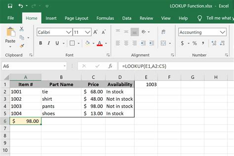
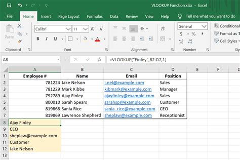
Using VLOOKUP Function

The VLOOKUP function is one of the most commonly used functions in Excel for looking up values in a table.

=VLOOKUP(A2, B:B, 1, FALSE)

A2 is the cell containing the value you want to look up.
B:B is the range where you want to search for the value.
1 indicates that you want to return a value from the first column of the range (in this case, column B itself).
FALSE means you're looking for an exact match.

If the value is found, VLOOKUP returns the value itself (since we're returning from the first column). If not found, it returns a #N/A error. You can wrap this in an IFERROR function to return a custom message instead of the error.

=IFERROR(VLOOKUP(A2, B:B, 1, FALSE), "Not Found")

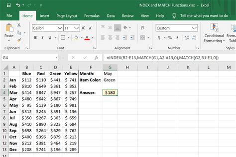
Using INDEX/MATCH Function

The INDEX/MATCH function combination is often preferred over VLOOKUP because it's more flexible and can look up values from any column, not just to the right of the lookup column.

=IFERROR(INDEX(B:B, MATCH(A2, B:B, 0)), "Not Found")

A2 is the value to look up.
B:B is the range to search in.
MATCH(A2, B:B, 0) finds the relative position of A2 in column B. The 0 means an exact match is required.
INDEX(B:B,...) returns the value at the position found by MATCH.

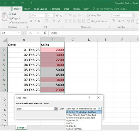
Using Conditional Formatting

If you want to visually highlight cells in column A that exist in column B without using formulas, you can use Conditional Formatting.

Select the cells in column A you want to format.
Go to the "Home" tab, find the "Styles" group, and click on "Conditional Formatting."
Choose "New Rule."
Select "Use a formula to determine which cells to format."
Enter the formula: =COUNTIF(B:B, A1) > 0 (assuming A1 is the first cell in your selection).
Click "Format" and choose how you want to highlight the cells.
Click "OK" to apply the rule.

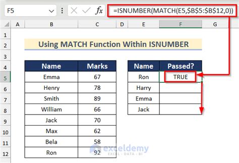
Using ISNUMBER and MATCH

Another approach is to use the combination of ISNUMBER and MATCH functions.

=ISNUMBER(MATCH(A2, B:B, 0))

This formula returns TRUE if the value in A2 is found in column B and FALSE otherwise. You can use this formula within an IF statement to return custom messages.

=IF(ISNUMBER(MATCH(A2, B:B, 0)), "Found", "Not Found")

Gallery of Excel Lookup Functions

Advanced Lookup Techniques

For more complex lookups, such as looking up values with multiple criteria or performing lookups in multiple columns, you might need to use more advanced techniques, including:

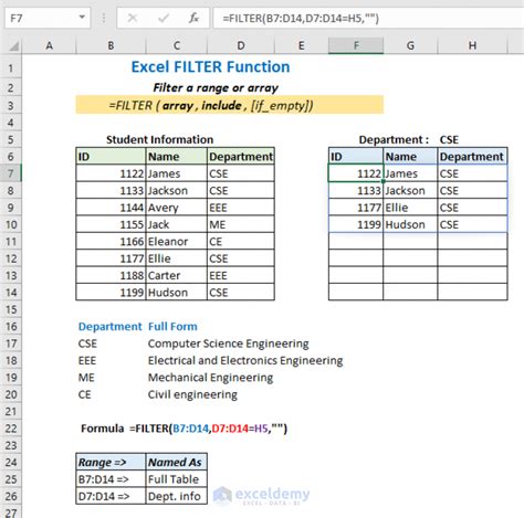
Using the FILTER function (available in Excel 2019 and later versions) for dynamic arrays.
Combining INDEX/MATCH with multiple criteria.
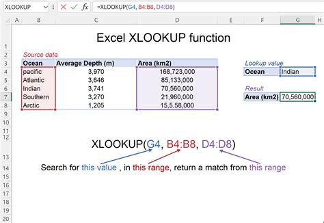
Utilizing the XLOOKUP function (available in Excel 2019 and later versions) for simpler and more efficient lookups.

Gallery of Excel Functions

Excel Functions Gallery

FAQs

What is the difference between VLOOKUP and INDEX/MATCH?

VLOOKUP looks up a value in the first column of a specified range and returns a value in the same row from another column. INDEX/MATCH offers more flexibility, allowing you to look up a value in any column and return a value from any other column, not just to the right of the lookup column.

How do I handle #N/A errors in lookup functions?

You can use the IFERROR function to return a custom message instead of the #N/A error. For example, =IFERROR(VLOOKUP(A2, B:B, 1, FALSE), "Not Found").

Can I use lookup functions with multiple criteria?

Yes, you can use the INDEX/MATCH function combination with multiple criteria by using the MATCH function twice, once for each criterion, and then using the INDEX function to return the value. Alternatively, you can use the FILTER function in newer versions of Excel for more complex and dynamic lookups.

In conclusion, checking if a value from one column exists in another column in Excel is a versatile task that can be accomplished through various methods, each with its own advantages and suitable scenarios. Whether you prefer the simplicity of VLOOKUP, the flexibility of INDEX/MATCH, or the visual approach of conditional formatting, Excel provides a range of tools to help you efficiently manage and analyze your data. By mastering these lookup techniques, you can significantly enhance your productivity and data analysis capabilities in Excel.

We hope this comprehensive guide has been helpful in your journey to become more proficient in Excel. Feel free to share your experiences, ask questions, or suggest topics you'd like to see covered in future articles. Your engagement is what drives us to create more informative and useful content for our readers.