Xlookup Formula In Cell B3

The Xlookup formula is a powerful and versatile tool in Excel that allows users to search for a value in a table and return a corresponding value from another column. In this article, we will delve into the world of Xlookup, exploring its importance, benefits, and practical applications. Whether you are a seasoned Excel user or just starting out, this article will provide you with a comprehensive understanding of the Xlookup formula and how to use it effectively.

The Xlookup formula is a game-changer for anyone who works with data in Excel. It simplifies the process of searching for and retrieving data, making it an essential tool for data analysis and manipulation. With Xlookup, you can quickly and easily find the data you need, saving you time and increasing your productivity. In this article, we will explore the benefits of using Xlookup, including its ease of use, flexibility, and accuracy.

One of the key advantages of Xlookup is its ability to search for values in a table and return corresponding values from another column. This makes it ideal for tasks such as data lookup, data validation, and data analysis. For example, suppose you have a table with customer names, addresses, and phone numbers, and you want to find the phone number of a specific customer. With Xlookup, you can simply enter the customer's name in a cell, and the formula will return the corresponding phone number.

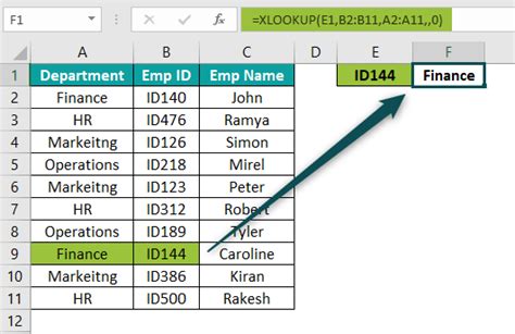
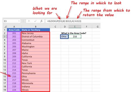
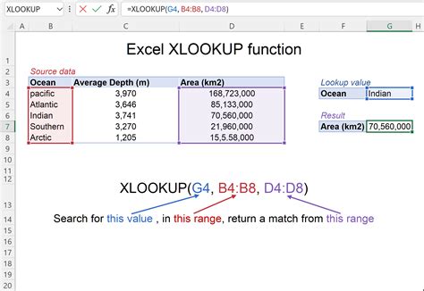
Xlookup Formula Syntax

The Xlookup formula syntax is simple and easy to use. The basic syntax is: Xlookup (lookup value, lookup array, return array, [if not found], [match mode], [search mode]). The lookup value is the value you want to search for, the lookup array is the range of cells that contains the values you want to search, the return array is the range of cells that contains the values you want to return, and the [if not found] argument is the value to return if the lookup value is not found.

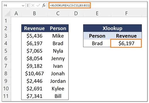
How to Use Xlookup Formula

Using the Xlookup formula is straightforward. Simply enter the formula in the cell where you want to display the result, and then press Enter. For example, suppose you want to find the phone number of a customer named John Smith. You can enter the following formula in cell B3: =Xlookup(A2, A:B, 2, "Not found"). In this formula, A2 is the cell that contains the customer's name, A:B is the range of cells that contains the customer names and phone numbers, 2 is the column number that contains the phone numbers, and "Not found" is the value to return if the customer's name is not found.

Xlookup Formula Benefits

The Xlookup formula has several benefits that make it a powerful tool for data analysis and manipulation. Some of the benefits include: * Easy to use: The Xlookup formula is simple and easy to use, even for users who are new to Excel. * Flexible: The Xlookup formula can be used to search for values in a variety of data ranges, including tables, ranges, and arrays. * Accurate: The Xlookup formula returns accurate results, even when dealing with large datasets. * Fast: The Xlookup formula is fast and efficient, making it ideal for tasks that require quick data lookup and retrieval.

Xlookup Formula Examples

Here are some examples of how to use the Xlookup formula: * Example 1: Find the phone number of a customer named John Smith. =Xlookup(A2, A:B, 2, "Not found") * Example 2: Find the address of a customer named Jane Doe. =Xlookup(A3, A:C, 3, "Not found") * Example 3: Find the sales total for a specific region. =Xlookup(B2, A:B, 2, "Not found")

Xlookup Formula Tips and Tricks

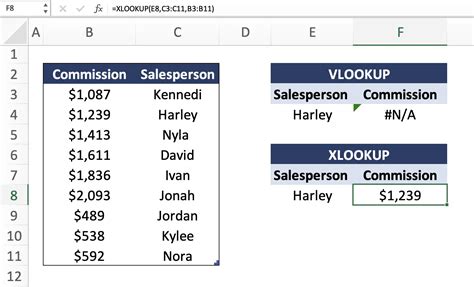
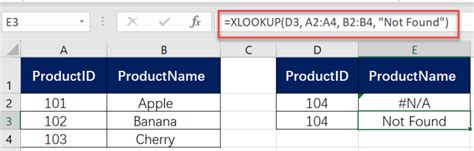
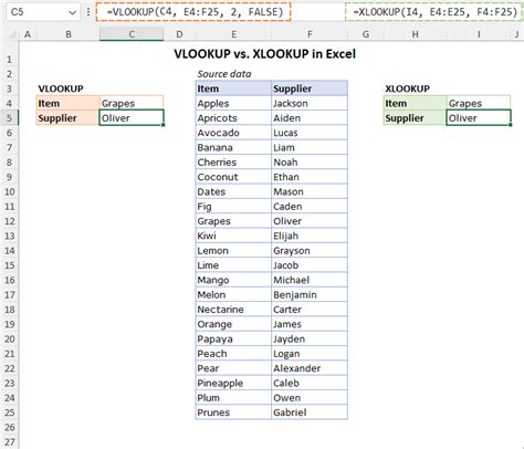
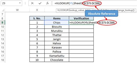
Here are some tips and tricks for using the Xlookup formula: * Use absolute references: When using the Xlookup formula, it's a good idea to use absolute references for the lookup array and return array. This ensures that the formula returns the correct results, even when the data range changes. * Use named ranges: Named ranges can make it easier to use the Xlookup formula, especially when working with large datasets. Simply define a named range for the lookup array and return array, and then use the named range in the formula. * Use error handling: The Xlookup formula returns a #N/A error if the lookup value is not found. To avoid this, you can use error handling functions such as IFERROR or IFNA.

Xlookup Formula vs Vlookup Formula

The Xlookup formula is similar to the Vlookup formula, but it has some key differences. The Vlookup formula searches for a value in a table and returns a corresponding value from another column, but it can be slow and inefficient, especially when dealing with large datasets. The Xlookup formula, on the other hand, is faster and more efficient, making it ideal for tasks that require quick data lookup and retrieval.

Xlookup Formula Best Practices

Here are some best practices for using the Xlookup formula: * Use the Xlookup formula instead of the Vlookup formula whenever possible. * Use absolute references for the lookup array and return array. * Use named ranges to make it easier to use the Xlookup formula. * Use error handling functions to avoid #N/A errors.

Xlookup Formula Common Errors

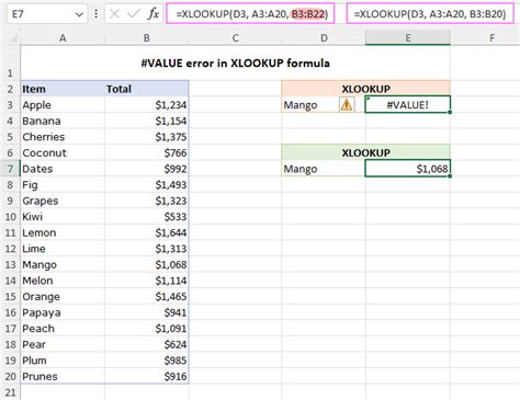
Here are some common errors that can occur when using the Xlookup formula: * #N/A error: This error occurs when the lookup value is not found in the lookup array. * #VALUE! error: This error occurs when the return array is not a valid range. * #REF! error: This error occurs when the lookup array or return array is not a valid range.

Xlookup Formula Troubleshooting

Here are some troubleshooting tips for common Xlookup formula errors: * Check the lookup value: Make sure the lookup value is correct and spelled correctly. * Check the lookup array: Make sure the lookup array is correct and contains the lookup value. * Check the return array: Make sure the return array is correct and contains the value you want to return.

Xlookup Formula Image Gallery

What is the Xlookup formula?

The Xlookup formula is a powerful and versatile tool in Excel that allows users to search for a value in a table and return a corresponding value from another column.

How do I use the Xlookup formula?

To use the Xlookup formula, simply enter the formula in the cell where you want to display the result, and then press Enter. The basic syntax is: Xlookup (lookup value, lookup array, return array, [if not found], [match mode], [search mode]).

What are the benefits of using the Xlookup formula?

The Xlookup formula has several benefits, including ease of use, flexibility, and accuracy. It is also faster and more efficient than the Vlookup formula, making it ideal for tasks that require quick data lookup and retrieval.

How do I troubleshoot common Xlookup formula errors?

To troubleshoot common Xlookup formula errors, check the lookup value, lookup array, and return array to ensure they are correct and valid. You can also use error handling functions such as IFERROR or IFNA to avoid #N/A errors.

What are some best practices for using the Xlookup formula?

Some best practices for using the Xlookup formula include using absolute references for the lookup array and return array, using named ranges to make it easier to use the formula, and using error handling functions to avoid #N/A errors.

In conclusion, the Xlookup formula is a powerful and versatile tool in Excel that can simplify the process of searching for and retrieving data. By understanding how to use the Xlookup formula, you can increase your productivity and accuracy, and make data analysis and manipulation easier and more efficient. We hope this article has provided you with a comprehensive understanding of the Xlookup formula and how to use it effectively. If you have any questions or comments, please don't hesitate to reach out. Share this article with your friends and colleagues, and help them to unlock the power of the Xlookup formula.