Excel Bar Chart Color Based On Value

Creating visually appealing and informative charts in Excel is a valuable skill for anyone working with data. One of the ways to make your charts more intuitive is by using colors to represent different values or categories. This can be particularly useful in bar charts, where the height of the bars already represents the magnitude of the data points. By coloring these bars based on their values, you can add an extra layer of information, making your chart more engaging and easier to understand.

In Excel, you can achieve this through various methods, including using conditional formatting, which is typically applied to cells, or by using more advanced chart customization options. Here, we'll explore how to color bars in a bar chart based on their values, focusing on methods that are both effective and easy to implement.

Understanding Your Data

Before you start, it's essential to understand the nature of your data. Are you working with categorical data where each category should have a distinct color, or are you dealing with numerical data where you want to represent different value ranges with different colors? This distinction will guide your approach to coloring your bar chart.

Using Conditional Formatting

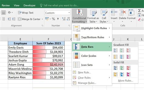
Conditional formatting is a powerful tool in Excel that allows you to highlight cells based on specific conditions. While it's primarily used for tables, you can also leverage it to color bars in a chart by first applying the formatting to the data range and then adjusting the chart settings to reflect these colors.

1. Select Your Data Range: Choose the cells containing the data you want to chart.
2. Apply Conditional Formatting: Go to the "Home" tab, find the "Styles" group, and click on "Conditional Formatting." Here, you can choose from various rules or use formulas to determine which cells to format.
3. Create a New Rule: Select "New Rule" and choose "Use a formula to determine which cells to format." Enter a formula that evaluates to true or false for each cell, based on the condition you want to apply (e.g., =A1>10 to format cells greater than 10).
4. Format: Click "Format" to choose the color you want to apply to cells meeting the condition. Click "OK" to apply the rule.

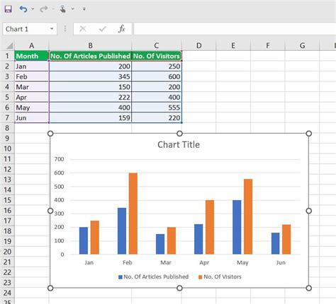
Creating the Bar Chart

After applying conditional formatting, create your bar chart:

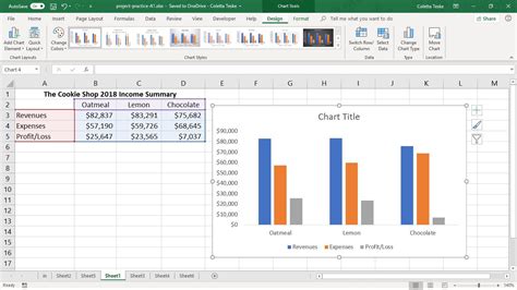
1. Select the Data: Including headers, select the range of cells with your data.
2. Insert Chart: Go to the "Insert" tab and click on "Bar Chart" to insert a basic bar chart.
3. Customize the Chart: Right-click on the chart and select "Select Data" to adjust the series and axes as needed.

However, simply applying conditional formatting to the data and then creating a chart might not directly translate the cell colors to the chart bars, as charts have their own formatting rules. For a more direct approach to coloring bars based on values within the chart itself, you might need to use a different method.

Directly Formatting the Chart

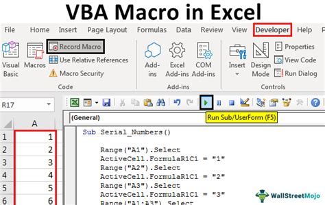
For a more precise control over the colors of your bars based on their values, you can use Excel's built-in chart formatting options, although this can be more complex and might require using macros for automation, especially if you have a large dataset.

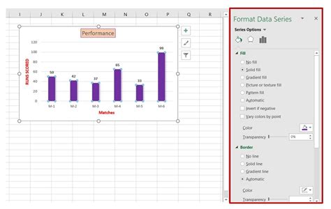
1. Select the Chart: Click on the chart to activate it.
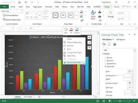
2. Format Data Series: With the chart selected, go to the "Format" tab under the "Chart Tools" contextual tab. Click on "Format Selection" or directly right-click on a data series (a group of bars) and select "Format Data Series."
3. Adjust Series Options: In the "Format Data Series" pane, you can adjust various options, including the fill color. However, to color based on value, you might need to use a workaround such as using multiple series for different value ranges, which can be cumbersome.

Advanced Techniques

For more advanced and dynamic coloring based on values, such as gradient colors or specific color scales, you might need to delve into Excel's more powerful features, like using VBA macros or add-ins that offer enhanced charting capabilities.

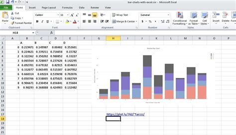
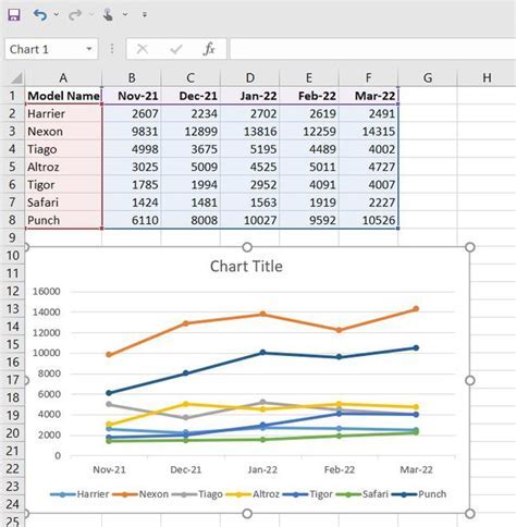
Gallery of Excel Bar Chart Examples

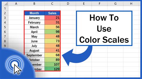
Gallery of Excel Chart Color Examples

Excel Chart Color Gallery

FAQs

How do I change the color of a bar in an Excel chart?

+

To change the color of a bar in an Excel chart, select the chart, then click on the "Format" tab under "Chart Tools." Choose "Format Selection" or right-click on the data series and select "Format Data Series" to adjust the fill color.

Can I automatically color bars based on their values in Excel?

+

Yes, you can use conditional formatting on the data range before creating the chart, but for direct control within the chart, you might need to use workarounds like multiple series or advanced techniques like VBA macros.

How do I create a bar chart in Excel?

+

Select your data range, go to the "Insert" tab, and click on "Bar Chart." Then, customize your chart as needed through the "Chart Tools" tabs.

In conclusion, while Excel provides various tools and features to customize your charts, including coloring bars based on their values, some methods might require creativity or diving into more advanced techniques. By understanding the capabilities and limitations of Excel's charting tools, you can create more informative and visually appealing charts that effectively communicate your data insights. Whether you're working with simple datasets or complex data analyses, mastering the art of chart customization in Excel can significantly enhance your data presentation and analysis capabilities.