Excel Conditional Formatting Color Based

Conditional formatting in Excel is a powerful tool that allows users to highlight cells based on specific conditions, making it easier to analyze and understand data. One of the most common uses of conditional formatting is to apply different colors to cells based on their values. This can help to draw attention to important information, identify trends, and make data more visually appealing. In this article, we will explore the different ways to use Excel conditional formatting color based, including the benefits, working mechanisms, and steps to apply it.

Excel conditional formatting color based can be used in a variety of situations, such as highlighting cells that contain specific text, numbers, or dates. It can also be used to highlight cells that are above or below a certain threshold, or to identify cells that contain errors. By applying different colors to cells based on their values, users can quickly and easily identify patterns and trends in their data, making it easier to make informed decisions.

Benefits of Excel Conditional Formatting Color Based

The benefits of using Excel conditional formatting color based are numerous. Some of the most significant advantages include:

Improved data visualization: By applying different colors to cells based on their values, users can quickly and easily identify patterns and trends in their data.
Increased productivity: Conditional formatting can save users a significant amount of time and effort, as it eliminates the need to manually review and highlight cells.
Enhanced decision-making: By highlighting important information and identifying trends, conditional formatting can help users make more informed decisions.
Simplified data analysis: Conditional formatting can make it easier to analyze large datasets, by drawing attention to key information and trends.

Working Mechanisms of Excel Conditional Formatting Color Based

The working mechanisms of Excel conditional formatting color based are relatively straightforward. To apply conditional formatting, users simply need to select the cells they want to format, and then choose the conditions they want to apply. Excel will then automatically apply the formatting to the selected cells, based on the conditions specified.

Some of the most common types of conditional formatting include:

Highlighting cells that contain specific text or numbers
Highlighting cells that are above or below a certain threshold
Highlighting cells that contain errors
Highlighting cells that are duplicates or unique

Steps to Apply Excel Conditional Formatting Color Based

To apply Excel conditional formatting color based, follow these steps:

Select the cells you want to format.
Go to the Home tab in the Excel ribbon.
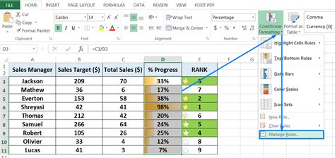
Click on the Conditional Formatting button in the Styles group.
Choose the type of formatting you want to apply, such as Highlight Cells Rules or Top/Bottom Rules.
Select the condition you want to apply, such as "Greater Than" or "Contains".
Specify the value or threshold you want to use.
Choose the format you want to apply, such as a specific color or font style.
Click OK to apply the formatting.

Practical Examples of Excel Conditional Formatting Color Based

Here are some practical examples of how to use Excel conditional formatting color based:

Highlighting cells that contain specific text: Suppose you have a list of customer names, and you want to highlight all the cells that contain the name "John". You can use the "Contains" condition to apply a specific color to all the cells that contain the name "John".
Highlighting cells that are above or below a certain threshold: Suppose you have a list of sales figures, and you want to highlight all the cells that are above $10,000. You can use the "Greater Than" condition to apply a specific color to all the cells that are above $10,000.
Highlighting cells that contain errors: Suppose you have a list of numbers, and you want to highlight all the cells that contain errors. You can use the "Errors" condition to apply a specific color to all the cells that contain errors.

Advanced Techniques for Excel Conditional Formatting Color Based

Advanced Techniques for Conditional Formatting

There are several advanced techniques you can use to take your Excel conditional formatting color based to the next level. Some of these techniques include:

Using multiple conditions: You can use multiple conditions to apply different formats to different cells.
Using formulas: You can use formulas to apply conditional formatting based on complex conditions.
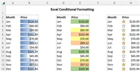
Using icons: You can use icons to apply conditional formatting, such as arrows or flags.
Using data bars: You can use data bars to apply conditional formatting, such as progress bars or thermometers.

Common Mistakes to Avoid When Using Excel Conditional Formatting Color Based

Here are some common mistakes to avoid when using Excel conditional formatting color based:

Not selecting the correct cells: Make sure to select the correct cells before applying conditional formatting.
Not specifying the correct condition: Make sure to specify the correct condition, such as "Greater Than" or "Contains".
Not choosing the correct format: Make sure to choose the correct format, such as a specific color or font style.
Not testing the formatting: Make sure to test the formatting to ensure it is working correctly.

Best Practices for Using Excel Conditional Formatting Color Based

Best Practices for Conditional Formatting

Here are some best practices to keep in mind when using Excel conditional formatting color based:

Keep it simple: Avoid using too many conditions or formats, as this can make the data difficult to read.
Use consistent formatting: Use consistent formatting throughout the workbook, to make it easier to read and understand.
Test the formatting: Test the formatting to ensure it is working correctly.
Document the formatting: Document the formatting, so that others can understand how it was applied.

Gallery of Excel Conditional Formatting Color Based

Excel Conditional Formatting Color Based Image Gallery

Conditional Formatting Color Based Example 1

Conditional Formatting Color Based Example 2

Conditional Formatting Color Based Example 3

Conditional Formatting Color Based Example 4

Conditional Formatting Color Based Example 5

Conditional Formatting Color Based Example 6

Conditional Formatting Color Based Example 7

Conditional Formatting Color Based Example 8

Conditional Formatting Color Based Example 9

Conditional Formatting Color Based Example 10

What is Excel conditional formatting color based?

Excel conditional formatting color based is a feature that allows users to highlight cells based on specific conditions, making it easier to analyze and understand data.

How do I apply Excel conditional formatting color based?

To apply Excel conditional formatting color based, select the cells you want to format, go to the Home tab, click on the Conditional Formatting button, and choose the type of formatting you want to apply.

What are the benefits of using Excel conditional formatting color based?

The benefits of using Excel conditional formatting color based include improved data visualization, increased productivity, enhanced decision-making, and simplified data analysis.

In summary, Excel conditional formatting color based is a powerful tool that can help users to analyze and understand data more effectively. By applying different colors to cells based on their values, users can quickly and easily identify patterns and trends, make informed decisions, and simplify data analysis. With its many benefits and advanced techniques, Excel conditional formatting color based is an essential feature for anyone who works with data in Excel. We hope this article has provided you with a comprehensive understanding of Excel conditional formatting color based, and we encourage you to try it out for yourself. If you have any questions or comments, please don't hesitate to reach out. Share this article with your friends and colleagues, and help them to unlock the full potential of Excel conditional formatting color based.