Intro
Highlighting cells based on another cell's value is a common requirement in spreadsheet applications like Microsoft Excel, Google Sheets, or LibreOffice Calc. This feature allows users to dynamically format cells based on conditions, making data analysis and visualization more efficient. In this article, we'll explore how to achieve this in various spreadsheet applications, focusing on the benefits, working mechanisms, steps, and practical examples.
The ability to highlight cells based on another cell's value is crucial for data analysis, as it enables users to quickly identify trends, patterns, or anomalies within their data sets. This feature is particularly useful in financial analysis, where cells might need to be highlighted based on budget thresholds, in inventory management, where stock levels might trigger specific formatting, or in any scenario where data comparison and visualization are key.
Why Highlight Cells Based on Another Cell's Value?
Highlighting cells based on another cell's value offers several benefits, including enhanced data readability, easier identification of critical data points, and the ability to automate the formatting process based on live data. This feature is a part of what's known as conditional formatting, a powerful tool in spreadsheet applications that allows users to apply specific formats to cells depending on the cell contents.
How to Highlight Cells Based on Another Cell's Value

The process of highlighting cells based on another cell's value involves selecting the cells you want to format, defining the condition based on another cell, and then applying the desired format. Here's a step-by-step guide for Microsoft Excel and Google Sheets:
- Select the Cells: Choose the range of cells you want to apply the formatting to.
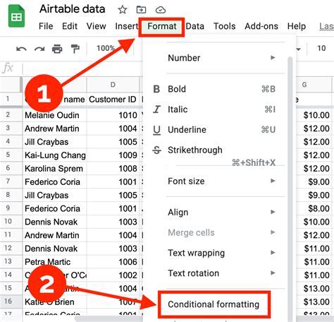
- Open Conditional Formatting: In Excel, go to the "Home" tab and click on "Conditional Formatting." In Google Sheets, select "Format" > "Conditional formatting."
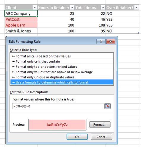
- Define the Rule: Select "New Rule" in Excel or "Add another rule" in Google Sheets. Choose "Use a formula to determine which cells to format" and enter your condition. For example, if you want to highlight cells in column A based on values in column B, your formula might look like
=B1>10, assuming you're starting from row 1. - Format the Cells: Click on "Format" and choose how you want the cells to appear when the condition is met (e.g., fill color, font color).
- Apply the Rule: Click "OK" to apply your rule. The selected cells will now change format based on the values in the other cells.
Practical Examples and Applications

- Financial Analysis: Highlight expenses exceeding a certain threshold to quickly identify areas for cost reduction.
- Inventory Management: Use conditional formatting to highlight low stock levels, prompting reordering.
- Grading: In educational settings, format cells to display grades based on score ranges.
Benefits of Conditional Formatting
The benefits of conditional formatting include:
- Enhanced Readability: Quickly identify important information.
- Automated Analysis: Reduce manual analysis time by automatically highlighting critical data points.
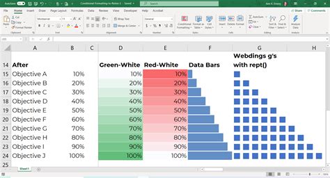
- Dynamic Visualization: As data changes, so does the formatting, providing a live view of your data's status.
Common Conditional Formatting Rules
Some common rules include highlighting cells based on:
- Greater Than:
=A1>10 - Less Than:
=A1<10 - Equal To:
=A1=10 - Text Contains:
=ISNUMBER(SEARCH("text",A1))
Advanced Conditional Formatting Techniques

For more complex scenarios, users can combine conditions, use nested formulas, or apply formatting to entire rows based on a single cell's value. Advanced techniques might include:
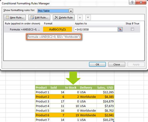
- Using AND, OR Functions: Combining multiple conditions, e.g.,
=AND(A1>10, B1="Yes"). - Applying to Entire Rows: Highlighting a row based on a condition in one column, useful for distinguishing between different categories of data.
Gallery of Conditional Formatting Examples
Conditional Formatting Image Gallery


What is Conditional Formatting?
+Conditional formatting is a feature in spreadsheet applications that allows users to format cells based on specific conditions or criteria.
How Do I Apply Conditional Formatting?
+Select the cells you want to format, open the conditional formatting menu, define your rule, and apply the format.
Can I Use Conditional Formatting with Multiple Conditions?
+Yes, you can combine conditions using AND, OR functions to create more complex rules for formatting cells.
In conclusion, highlighting cells based on another cell's value is a powerful feature in spreadsheet applications that enhances data analysis, visualization, and readability. By mastering conditional formatting, users can automate the process of identifying critical data points, trends, and patterns, making their work more efficient and effective. Whether you're working with financial data, managing inventory, or analyzing student performance, conditional formatting is a tool that can significantly improve your workflow and insights. We invite you to explore more about conditional formatting, share your experiences with it, and ask any questions you might have about implementing this feature in your spreadsheet applications.