5 Ways Freeze Rows

Freezing rows in spreadsheets is a crucial feature that allows users to keep specific rows visible while scrolling through the rest of the data. This can be particularly useful for headers, summary rows, or any other row that provides context to the data below or above it. Here are five ways to freeze rows, along with explanations and examples to help you understand how to apply these methods in different scenarios.

Freezing rows can significantly enhance your productivity and data analysis capabilities. Whether you're working with Microsoft Excel, Google Sheets, or another spreadsheet software, the ability to lock certain rows in place can make navigating large datasets much easier. This feature is especially beneficial when dealing with complex spreadsheets that contain numerous rows and columns, making it difficult to keep track of your position within the data without a fixed point of reference.

The importance of freezing rows cannot be overstated, particularly in professional settings where data analysis is a critical component of decision-making processes. By keeping key information, such as column headers or summary statistics, always in view, analysts can more efficiently interpret data trends and patterns. Moreover, this feature simplifies the process of comparing data across different rows, as the reference points remain constant, reducing the likelihood of errors that might arise from scrolling back and forth to check headers or other important information.

Understanding Freeze Rows

Before diving into the methods of freezing rows, it's essential to understand the concept and its applications. Freezing rows allows you to divide your spreadsheet into two sections: a frozen section that remains visible at all times and a scrollable section where you can navigate through your data. This division can be customized to fit the specific needs of your project, whether it involves freezing a single row at the top for headers or multiple rows for more complex data summaries.

Method 1: Freezing Top Row

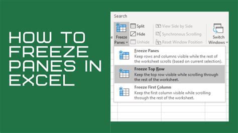
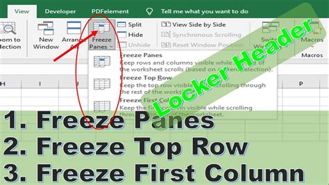
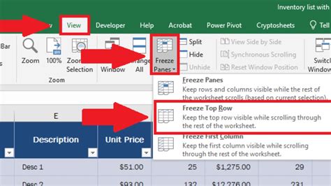
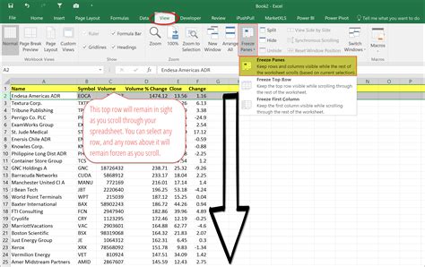
One of the most common methods of freezing rows is to freeze the top row. This is particularly useful for keeping column headers in view as you scroll down through your data. To freeze the top row in Microsoft Excel, for example, you can go to the "View" tab, click on "Freeze Panes," and then select "Freeze Top Row." This action will lock the first row in place, allowing you to scroll through the rest of your spreadsheet without losing sight of your column headers.

Steps to Freeze Top Row in Google Sheets

1. Select the row below the one you want to freeze.
2. Go to the "View" menu.
3. Hover over "Freeze," and then select the number of rows you want to freeze.

This method is straightforward and applies to most spreadsheet applications with minor variations in the steps.

Method 2: Freezing Multiple Rows

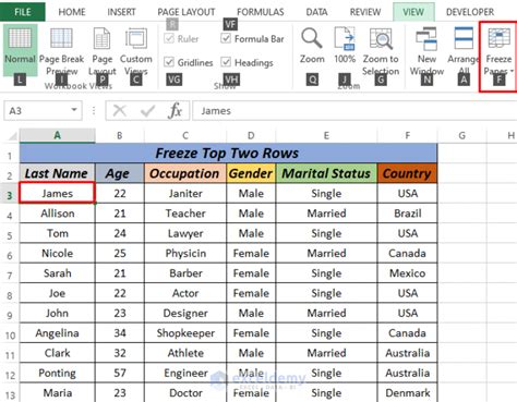
For more complex datasets or summaries, you might need to freeze multiple rows. This could be the case if you have multiple header rows or if you're working with a summary section that you want to keep in view. To freeze multiple rows, you follow a similar process as freezing a single row, but you select the row below the last row you wish to freeze before applying the freeze command.

Benefits of Freezing Multiple Rows

• Enhanced data interpretation by keeping complex headers or summaries in view.
• Improved navigation through large datasets.
• Reduced errors from misinterpreting data due to lost context.

Method 3: Freezing Rows in Google Sheets

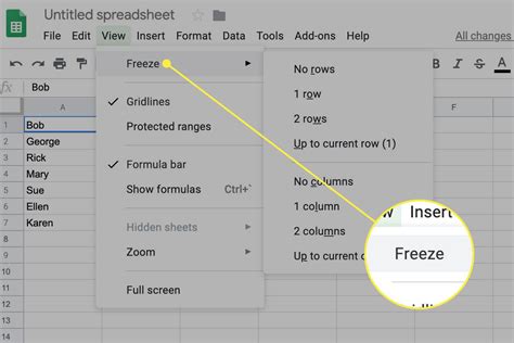
Google Sheets offers a convenient way to freeze rows directly from the menu. By selecting the row below the one you want to freeze, going to the "View" menu, and selecting "Freeze," you can choose how many rows to freeze. This method is intuitive and works well for collaborative projects where team members might need to analyze data together in real-time.

Collaborative Benefits

• Real-time collaboration: Multiple users can view and analyze the same data simultaneously.
• Consistent view: Freezing rows ensures that all collaborators have the same reference points, enhancing communication and reducing misunderstandings.

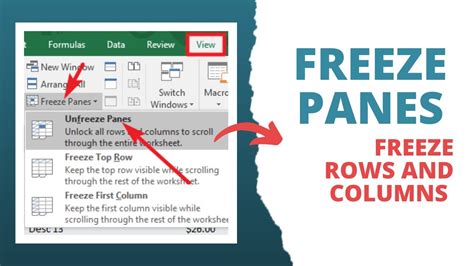
Method 4: Using Freeze Panes

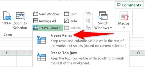
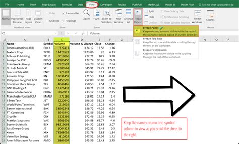
For more customized views, you can use the "Freeze Panes" feature. This allows you to freeze both rows and columns, creating a split-screen effect where one section of your spreadsheet remains fixed while you scroll through another. This is particularly useful for comparing data across different parts of your spreadsheet or for keeping a reference section in view.

Customization Options

• Freeze rows and columns: Create a customized view that suits your analysis needs.
• Split-screen view: Enhance data comparison by keeping reference data in view.

Method 5: Advanced Freezing Techniques

For complex spreadsheets, advanced freezing techniques can be employed. This includes freezing rows and columns in combination, using multiple freeze points, or even utilizing macros and scripts to dynamically adjust frozen areas based on the data. These techniques require a deeper understanding of spreadsheet functions and programming but can offer unparalleled flexibility and customization.

Advanced Applications

• Dynamic freezing: Use macros or scripts to adjust frozen areas based on data changes.
• Multi-point freezing: Freeze multiple, non-contiguous rows or columns for complex data analysis.

Freeze Rows Image Gallery

What is the purpose of freezing rows in a spreadsheet?

+

The purpose of freezing rows is to keep specific rows visible at all times, typically for headers or summaries, making data analysis and navigation easier.

How do I freeze rows in Google Sheets?

+

To freeze rows in Google Sheets, select the row below the one you want to freeze, go to the "View" menu, hover over "Freeze," and select the number of rows you want to freeze.

Can I freeze both rows and columns in a spreadsheet?

+

Yes, you can freeze both rows and columns using the "Freeze Panes" feature, which allows for a customized view that suits your data analysis needs.

In conclusion, freezing rows is a powerful tool in spreadsheet applications that can significantly enhance your ability to analyze and navigate through data. By understanding the different methods of freezing rows and applying them appropriately, you can improve your productivity and reduce the complexity of working with large datasets. Whether you're a professional data analyst or simply managing personal finances, mastering the art of freezing rows can make a substantial difference in how you interact with and understand your data. We invite you to share your experiences with freezing rows, ask questions about the methods discussed, or explore more advanced techniques for customizing your spreadsheet views.