Excel Conditional Format Compare Two Columns

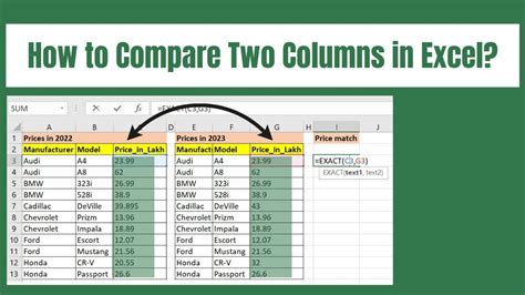
When working with Excel, comparing two columns is a common task, especially for identifying duplicates, differences, or matches between two sets of data. Excel's Conditional Formatting feature allows you to highlight cells based on specific conditions, making it easier to visualize and analyze data. Here, we will explore how to use Conditional Formatting to compare two columns in Excel, highlighting the similarities and differences between them.

Excel's Conditional Formatting offers a variety of options to compare data, including formulas that can be used to compare two columns. This feature is particularly useful for data analysis, as it allows you to visually distinguish between cells that meet certain conditions, such as being greater than, less than, or equal to a value in another column.

To get started with comparing two columns using Conditional Formatting, you first need to select the range of cells you want to format. This could be an entire column or a specific range within a column. Once you've selected your range, you can access the Conditional Formatting options through the Home tab on the Excel ribbon.

How to Compare Two Columns Using Conditional Formatting

Comparing two columns involves creating a rule that checks for a condition between the cells in one column and the cells in another. This can be achieved by using a formula within the Conditional Formatting dialog box. Here’s a step-by-step guide:

1. Select the Range: Choose the cells in one of the columns you want to compare.
2. Open Conditional Formatting: Go to the Home tab, find the Styles group, and click on Conditional Formatting.
3. New Rule: Select "New Rule" to create a custom format.
4. Use a Formula: Choose "Use a formula to determine which cells to format."
5. Enter the Formula: Here, you can enter a formula that compares the two columns. For example, if you want to highlight cells in column A that are equal to cells in column B, you could use a formula like =A1=B1, assuming you're starting from row 1.
6. Format: Click the Format button to choose how you want to highlight the cells that meet the condition.
7. Apply: Click OK to apply the rule.

Common Formulas for Comparing Columns

When comparing two columns, you might use several types of formulas, depending on what you're trying to achieve. Here are a few examples:

• Exact Match: =A1=B1 highlights cells in column A that exactly match cells in column B.
• Not Equal: =A1<>B1 highlights cells in column A that do not match cells in column B.
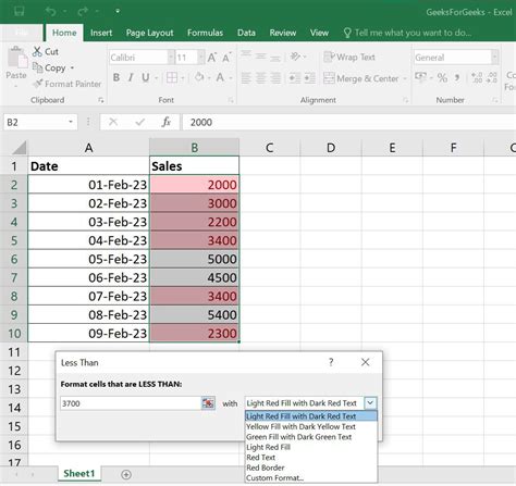
• Greater Than: =A1>B1 highlights cells in column A that are greater than cells in column B.
• Less Than: =A1<B1 highlights cells in column A that are less than cells in column B.

Remember, when you enter a formula in the Conditional Formatting dialog, it applies to the first cell of your selected range. Excel automatically adjusts the formula for each cell in the range.

Benefits of Using Conditional Formatting

Conditional Formatting offers several benefits when comparing two columns:

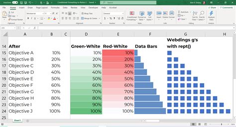
• Visual Analysis: It allows for quick visual analysis of data by highlighting important trends or discrepancies.
• Ease of Use: The feature is relatively easy to use, even for those without extensive Excel knowledge.
• Flexibility: You can create various rules based on different conditions, making it highly adaptable to different data analysis needs.
• Dynamic Updates: When your data changes, the formatting updates automatically, reflecting the new conditions.

Best Practices for Conditional Formatting

To get the most out of Conditional Formatting when comparing two columns, consider the following best practices:

• Keep it Simple: Start with simple rules and gradually move to more complex ones as needed.
• Test Your Rules: Always test your conditional formatting rules on a small set of data before applying them to larger datasets.
• Use Clear and Consistent Formatting: Ensure that your formatting is easy to understand and consistent throughout your spreadsheet.

Common Challenges and Solutions

When using Conditional Formatting to compare two columns, you might encounter a few challenges:

• Formula Errors: Double-check your formulas for any syntax errors or incorrect references.
• Inconsistent Data: Ensure that the data in both columns is consistent in terms of formatting and content.
• Performance Issues: For very large datasets, Conditional Formatting might slow down your Excel performance. Consider applying rules to smaller ranges or using other data analysis tools.

Gallery of Conditional Formatting Examples

Conditional Formatting Image Gallery

What is Conditional Formatting in Excel?

+

Conditional Formatting is a feature in Excel that allows you to highlight cells based on specific conditions, making it easier to visualize and analyze data.

How do I compare two columns using Conditional Formatting?

+

To compare two columns, select the range of cells, go to Conditional Formatting, choose "New Rule," select "Use a formula to determine which cells to format," and enter a formula that compares the two columns.

What are some common formulas used for comparing columns?

+

Common formulas include `=A1=B1` for exact matches, `=A1<>B1` for non-matches, `=A1>B1` for greater than, and `=A1

In conclusion, Conditional Formatting is a powerful tool in Excel for comparing two columns and highlighting important trends or discrepancies in your data. By following the steps and tips outlined above, you can leverage this feature to enhance your data analysis capabilities. Whether you're looking to identify matches, differences, or specific conditions between two sets of data, Conditional Formatting provides a flexible and dynamic solution. Feel free to share your experiences or ask questions about using Conditional Formatting for comparing columns in the comments below.