Excel Pivot Table Top 10

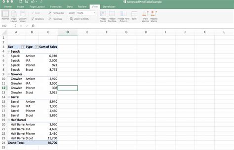
Excel Pivot Tables are a powerful tool for data analysis, allowing users to summarize, analyze, and visualize large datasets with ease. One of the most useful features of Pivot Tables is the ability to display the top 10 items in a particular field, making it easy to identify trends, patterns, and outliers in the data. In this article, we will explore the importance of Excel Pivot Tables and the Top 10 feature, and provide a step-by-step guide on how to use it.

The ability to analyze and understand large datasets is crucial in today's data-driven world. With the increasing amount of data being generated every day, it's becoming more challenging to make sense of it all. This is where Excel Pivot Tables come in, providing a powerful tool for data analysis and visualization. By using Pivot Tables, users can quickly and easily summarize and analyze large datasets, identify trends and patterns, and make informed decisions.

Pivot Tables are particularly useful for identifying the top 10 items in a particular field, such as the top 10 products by sales, the top 10 customers by revenue, or the top 10 regions by population. This information can be used to inform business decisions, identify areas for improvement, and optimize resources. In the following sections, we will explore the benefits of using Excel Pivot Tables and the Top 10 feature, and provide a step-by-step guide on how to use it.

Introduction to Excel Pivot Tables

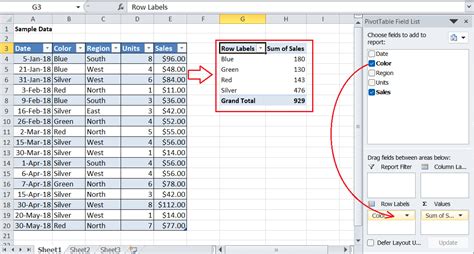
Excel Pivot Tables are a powerful tool for data analysis, allowing users to summarize, analyze, and visualize large datasets with ease. Pivot Tables are particularly useful for identifying trends, patterns, and outliers in the data, and can be used to inform business decisions, identify areas for improvement, and optimize resources. By using Pivot Tables, users can quickly and easily summarize and analyze large datasets, and make informed decisions.

Benefits of Using Excel Pivot Tables

The benefits of using Excel Pivot Tables are numerous, and include: * The ability to quickly and easily summarize and analyze large datasets * The ability to identify trends, patterns, and outliers in the data * The ability to inform business decisions, identify areas for improvement, and optimize resources * The ability to create interactive and dynamic reports that can be easily updated and refreshed * The ability to analyze and visualize data from multiple sources and formats

Using the Top 10 Feature in Excel Pivot Tables

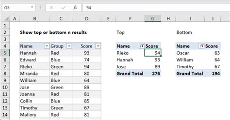
The Top 10 feature in Excel Pivot Tables allows users to display the top 10 items in a particular field, making it easy to identify trends, patterns, and outliers in the data. To use the Top 10 feature, follow these steps:

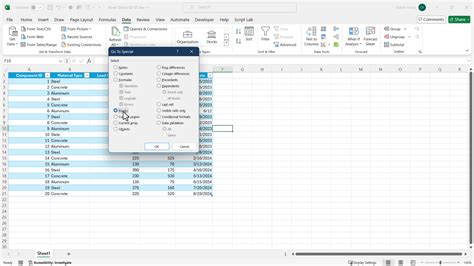
Create a Pivot Table by selecting a cell range and going to the "Insert" tab in the ribbon
Select the field that you want to display the top 10 items for, such as "Sales" or "Revenue"
Right-click on the field and select "Value Field Settings"
In the "Value Field Settings" dialog box, select the "Top 10" option
Enter the number of items that you want to display, such as 10
Click "OK" to apply the changes

Step-by-Step Guide to Using the Top 10 Feature

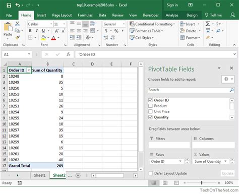
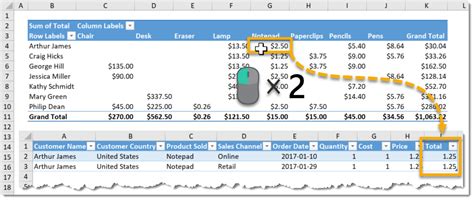
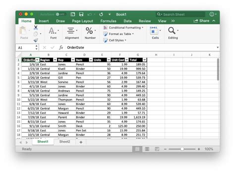
Here is a step-by-step guide to using the Top 10 feature in Excel Pivot Tables: * Select the cell range that contains the data that you want to analyze * Go to the "Insert" tab in the ribbon and select "PivotTable" * Select the field that you want to display the top 10 items for, such as "Sales" or "Revenue" * Right-click on the field and select "Value Field Settings" * In the "Value Field Settings" dialog box, select the "Top 10" option * Enter the number of items that you want to display, such as 10 * Click "OK" to apply the changes

Advanced Features of Excel Pivot Tables

Excel Pivot Tables have a number of advanced features that can be used to further analyze and visualize data. Some of these features include:

The ability to create multiple Pivot Tables from a single dataset
The ability to use multiple fields to create a Pivot Table
The ability to use filters to narrow down the data that is displayed in the Pivot Table
The ability to use slicers to select specific data points to display in the Pivot Table
The ability to create interactive and dynamic dashboards using Pivot Tables and other Excel tools

Using Multiple Fields to Create a Pivot Table

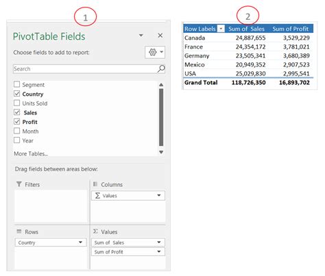
To use multiple fields to create a Pivot Table, follow these steps: * Select the cell range that contains the data that you want to analyze * Go to the "Insert" tab in the ribbon and select "PivotTable" * Select the first field that you want to use to create the Pivot Table * Right-click on the field and select "Value Field Settings" * In the "Value Field Settings" dialog box, select the "Add" option * Select the second field that you want to use to create the Pivot Table * Repeat the process until you have added all of the fields that you want to use

Best Practices for Using Excel Pivot Tables

Here are some best practices for using Excel Pivot Tables:

Use clear and concise field names to make it easy to understand the data
Use filters to narrow down the data that is displayed in the Pivot Table
Use slicers to select specific data points to display in the Pivot Table
Use multiple fields to create a Pivot Table to get a more detailed view of the data
Use the Top 10 feature to identify trends, patterns, and outliers in the data

Common Mistakes to Avoid When Using Excel Pivot Tables

Here are some common mistakes to avoid when using Excel Pivot Tables: * Not using clear and concise field names * Not using filters to narrow down the data that is displayed in the Pivot Table * Not using slicers to select specific data points to display in the Pivot Table * Not using multiple fields to create a Pivot Table * Not using the Top 10 feature to identify trends, patterns, and outliers in the data

Excel Pivot Table Image Gallery

What is an Excel Pivot Table?

An Excel Pivot Table is a powerful tool for data analysis, allowing users to summarize, analyze, and visualize large datasets with ease.

How do I create a Pivot Table in Excel?

To create a Pivot Table in Excel, select a cell range and go to the "Insert" tab in the ribbon, then select "PivotTable".

What is the Top 10 feature in Excel Pivot Tables?

The Top 10 feature in Excel Pivot Tables allows users to display the top 10 items in a particular field, making it easy to identify trends, patterns, and outliers in the data.

In conclusion, Excel Pivot Tables are a powerful tool for data analysis, and the Top 10 feature is a valuable asset for identifying trends, patterns, and outliers in the data. By following the steps outlined in this article, users can create a Pivot Table and use the Top 10 feature to gain insights into their data. We hope this article has been helpful in understanding the importance of Excel Pivot Tables and the Top 10 feature. If you have any questions or comments, please don't hesitate to reach out. Share this article with your friends and colleagues who may benefit from learning about Excel Pivot Tables and the Top 10 feature.