Intro
Master Excel Vlookup with two conditions using multiple criteria, index-match functions, and nested lookups to retrieve precise data, enhancing spreadsheet analysis and reporting capabilities.
The Vlookup function in Excel is a powerful tool used for looking up and retrieving data from a table based on a specific value. However, there are instances where you might need to look up data based on two conditions. Unfortunately, the traditional Vlookup function does not support this directly, but there are workarounds and alternative functions that can help achieve this.
In many cases, users find themselves in situations where they need to retrieve data from a large dataset based on multiple criteria. This could be for managing inventories, tracking sales, analyzing student performance, or any other scenario where data is organized in tables and needs to be filtered based on more than one condition.
To tackle this challenge, Excel offers several methods, including using the Index/Match function combination, which is more flexible than Vlookup, or utilizing the Xlookup function, which is available in newer versions of Excel and offers more straightforward lookup capabilities, including handling multiple lookup values.
Understanding the Vlookup Function
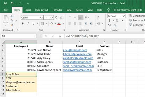
The Vlookup function is used to look up a value in a table and return a value from another column. The syntax for Vlookup is VLOOKUP(lookup_value, table_array, col_index_num, [range_lookup]). However, as mentioned, it does not inherently support looking up values based on two conditions without combining it with other functions.
Using Index/Match for Two Conditions
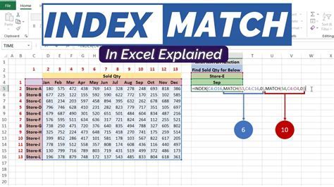
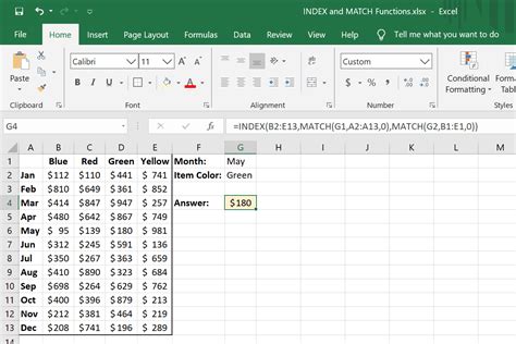
One of the most popular alternatives for looking up data with two conditions is using the Index/Match function combination. This method is highly flexible and can be used in a variety of scenarios. The formula typically looks something like this: =INDEX(return_range, MATCH(1, (condition1) * (condition2), 0)), where return_range is the range from which you want to return a value, and condition1 and condition2 are the criteria you're looking up.
For example, if you have a table with names in column A, ages in column B, and cities in column C, and you want to find the age of a person who lives in a specific city and has a specific name, you could use the following formula:
=INDEX(B:B, MATCH(1, (A:A="John") * (C:C="New York"), 0))
This formula looks for "John" in column A and "New York" in column C, and returns the corresponding age from column B.
Xlookup for Multiple Conditions

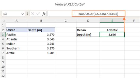
For users with Excel 2019 or later versions, including Office 365, the Xlookup function offers a more straightforward way to handle lookups with multiple conditions. The Xlookup function can look up a value and return a result from another column, and it also supports handling errors more elegantly than Vlookup.
The syntax for Xlookup with multiple conditions is XLOOKUP(lookup_value1, lookup_array1, lookup_value2, lookup_array2, return_array, [if_not_found], [match_mode], [search_mode]). However, for multiple conditions, you might still need to combine Xlookup with other functions or use the filter function in combination.
Using Filter Function

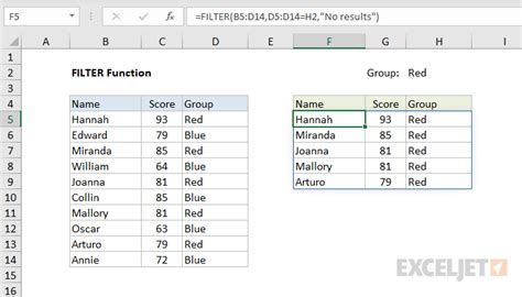
The Filter function, available in Excel 365 and later versions, allows you to filter a range of data based on criteria. You can use it to return values based on multiple conditions. The syntax is FILTER(array, include, [if_blank]), where array is the range of cells that you want to filter, and include specifies the criteria.
For example, to filter a table to show only rows where the name is "John" and the city is "New York", you could use:
=FILTER(B:B, (A:A="John") * (C:C="New York"))
This formula returns all ages from column B where the conditions are met.
Step-by-Step Guide to Implementing Two-Condition Lookup

- Prepare Your Data: Ensure your data is organized in a table format with clear headers.
- Choose Your Method: Decide whether to use Index/Match, Xlookup, or the Filter function based on your Excel version and preference.
- Identify Your Conditions: Clearly define the two conditions you want to look up.
- Apply the Formula: Use the appropriate formula based on the method you've chosen, adjusting the ranges and conditions as necessary.
- Test Your Formula: Ensure the formula returns the expected results and adjust as needed.
Gallery of Excel Lookup Functions
Excel Lookup Functions Image Gallery


Frequently Asked Questions
What is the main difference between Vlookup and Index/Match?
+Vlookup looks up a value in the first column of a table and returns a value in the same row from another column, whereas Index/Match offers more flexibility, including looking up values in any column and handling multiple conditions more easily.
How do I handle errors with the Xlookup function?
+Xlookup allows you to specify a value to return if the lookup value is not found, using the `[if_not_found]` argument. This can help in handling errors more elegantly than traditional Vlookup.
Can I use the Filter function for dynamic dashboards?
+Yes, the Filter function is very useful for creating dynamic dashboards that update automatically based on user-selected criteria. It's a powerful tool for data analysis and visualization in Excel.
In conclusion, while the traditional Vlookup function does not directly support looking up data with two conditions, Excel offers several alternative methods and functions that can achieve this, including the Index/Match combination, the Xlookup function, and the Filter function. By understanding and applying these methods, users can efficiently manage and analyze their data in Excel, making it a more powerful tool for their needs. If you have any questions or need further clarification on using these functions, feel free to ask in the comments below. Share your experiences with Excel lookup functions and how they've helped you in your data analysis tasks.