Intro
Discover 5 Google Sheets ranking formulas to simplify data analysis, including RANK, LARGE, SMALL, INDEX/MATCH, and OFFSET, for efficient data sorting and manipulation, improving spreadsheet productivity with these essential formulas.
The importance of ranking data in Google Sheets cannot be overstated, as it provides valuable insights and helps in making informed decisions. Ranking formulas are essential tools in data analysis, allowing users to compare and prioritize data points based on specific criteria. Whether you're a business owner looking to rank sales performance, a student trying to rank academic achievements, or an analyst seeking to rank data trends, Google Sheets offers a variety of ranking formulas to suit your needs. In this article, we will delve into five Google Sheets ranking formulas, exploring their applications, benefits, and step-by-step instructions on how to use them.
Google Sheets is a powerful and versatile tool that has become an indispensable part of modern data analysis. Its ability to handle complex data sets, perform calculations, and visualize information makes it an ideal platform for ranking data. With the help of ranking formulas, users can easily identify top performers, trends, and patterns in their data, enabling them to make data-driven decisions. The five ranking formulas discussed in this article are the RANK function, the RANK.AVG function, the RANK.EQ function, the LARGE function, and the SMALL function. Each of these formulas has its unique characteristics and applications, and understanding how to use them effectively is crucial for anyone working with data in Google Sheets.
The RANK function is one of the most commonly used ranking formulas in Google Sheets. It assigns a rank to each value in a list, based on its position in the sorted list. The RANK function is useful for identifying top performers, such as the top-selling products or the highest-scoring students. To use the RANK function, simply type "=RANK(value, range, [order])" in the formula bar, where "value" is the cell containing the value to be ranked, "range" is the range of cells containing the list of values, and "[order]" is an optional argument that specifies the sorting order. For example, if you want to rank the values in the range A1:A10 in descending order, you would use the formula "=RANK(A1, A1:A10, 0)".
Understanding the RANK Function
The RANK function is a straightforward and easy-to-use formula that provides valuable insights into your data. However, it has some limitations, such as not being able to handle tied values. In cases where two or more values are equal, the RANK function assigns the same rank to all tied values, skipping the next rank. For example, if you have two values tied for first place, the RANK function will assign a rank of 1 to both values, and the next value will be assigned a rank of 3.
Using the RANK.AVG Function
To overcome the limitation of the RANK function, you can use the RANK.AVG function, which assigns the average rank to tied values. The RANK.AVG function is similar to the RANK function, but it uses a different algorithm to handle tied values. To use the RANK.AVG function, simply type "=RANK.AVG(value, range, [order])" in the formula bar, where "value" is the cell containing the value to be ranked, "range" is the range of cells containing the list of values, and "[order]" is an optional argument that specifies the sorting order. For example, if you want to rank the values in the range A1:A10 in descending order using the RANK.AVG function, you would use the formula "=RANK.AVG(A1, A1:A10, 0)".Ranking Data with the RANK.EQ Function
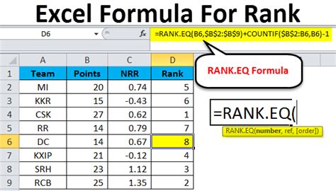
The RANK.EQ function is another useful ranking formula in Google Sheets. It assigns the same rank to tied values, without skipping any ranks. The RANK.EQ function is useful when you want to assign the same rank to tied values, without leaving any gaps in the ranking. To use the RANK.EQ function, simply type "=RANK.EQ(value, range, [order])" in the formula bar, where "value" is the cell containing the value to be ranked, "range" is the range of cells containing the list of values, and "[order]" is an optional argument that specifies the sorting order. For example, if you want to rank the values in the range A1:A10 in descending order using the RANK.EQ function, you would use the formula "=RANK.EQ(A1, A1:A10, 0)".
Using the LARGE Function
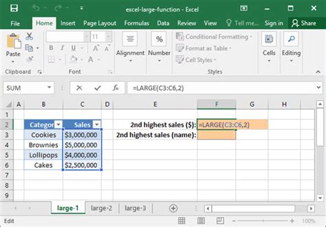
The LARGE function is a useful formula for ranking data in Google Sheets. It returns the nth largest value in a range of cells. The LARGE function is useful when you want to identify the top values in a list, such as the top 5 sales figures or the top 10 highest-scoring students. To use the LARGE function, simply type "=LARGE(range, n)" in the formula bar, where "range" is the range of cells containing the list of values, and "n" is the position of the value you want to return. For example, if you want to return the 5th largest value in the range A1:A10, you would use the formula "=LARGE(A1:A10, 5)".Ranking Data with the SMALL Function
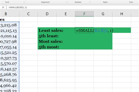
The SMALL function is similar to the LARGE function, but it returns the nth smallest value in a range of cells. The SMALL function is useful when you want to identify the bottom values in a list, such as the bottom 5 sales figures or the bottom 10 lowest-scoring students. To use the SMALL function, simply type "=SMALL(range, n)" in the formula bar, where "range" is the range of cells containing the list of values, and "n" is the position of the value you want to return. For example, if you want to return the 5th smallest value in the range A1:A10, you would use the formula "=SMALL(A1:A10, 5)".
Practical Examples of Ranking Formulas
Ranking formulas have a wide range of applications in real-life scenarios. For example, a business owner can use the RANK function to rank sales performance, identifying the top-selling products and the sales teams that need improvement. A student can use the RANK.AVG function to rank academic achievements, identifying the top-scoring students and the subjects that need more attention. An analyst can use the LARGE function to rank data trends, identifying the top trends and the areas that need more investment.Benefits of Using Ranking Formulas

The benefits of using ranking formulas in Google Sheets are numerous. They provide valuable insights into your data, enabling you to make informed decisions. They help you identify top performers, trends, and patterns in your data, allowing you to prioritize your efforts and resources. They also enable you to compare and contrast different data points, providing a comprehensive understanding of your data.
Steps to Use Ranking Formulas
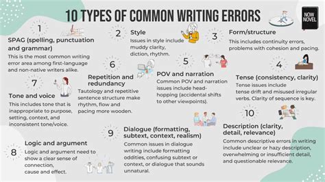
Using ranking formulas in Google Sheets is straightforward. Here are the steps to follow: * Select the cell where you want to display the ranked value. * Type the ranking formula, such as "=RANK(value, range, [order])". * Press Enter to execute the formula. * Adjust the formula as needed to suit your specific needs.Common Errors and Troubleshooting
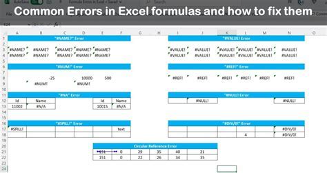
Common errors and troubleshooting are essential aspects of using ranking formulas in Google Sheets. Here are some common errors to watch out for:
- Incorrect syntax: Make sure to type the formula correctly, including the parentheses and commas.
- Invalid arguments: Ensure that the arguments you pass to the formula are valid, such as a range of cells or a value.
- Division by zero: Avoid dividing by zero, as this will result in an error.
Best Practices for Using Ranking Formulas
Best practices for using ranking formulas in Google Sheets include: * Using the correct formula for your specific needs. * Ensuring that your data is accurate and up-to-date. * Using conditional formatting to highlight ranked values. * Creating a table of contents to navigate your spreadsheet.Gallery of Ranking Formulas
Ranking Formulas Image Gallery


Frequently Asked Questions
What is the RANK function in Google Sheets?
+The RANK function in Google Sheets assigns a rank to each value in a list, based on its position in the sorted list.
How do I use the RANK.AVG function in Google Sheets?
+To use the RANK.AVG function in Google Sheets, simply type "=RANK.AVG(value, range, [order])" in the formula bar, where "value" is the cell containing the value to be ranked, "range" is the range of cells containing the list of values, and "[order]" is an optional argument that specifies the sorting order.
What is the difference between the RANK and RANK.EQ functions in Google Sheets?
+The RANK function assigns a rank to each value in a list, based on its position in the sorted list, while the RANK.EQ function assigns the same rank to tied values, without skipping any ranks.
How do I use the LARGE function in Google Sheets?
+To use the LARGE function in Google Sheets, simply type "=LARGE(range, n)" in the formula bar, where "range" is the range of cells containing the list of values, and "n" is the position of the value you want to return.
What are some common errors to watch out for when using ranking formulas in Google Sheets?
+Common errors to watch out for when using ranking formulas in Google Sheets include incorrect syntax, invalid arguments, and division by zero.
In conclusion, ranking formulas are essential tools in Google Sheets, providing valuable insights and helping users make informed decisions. By understanding how to use the RANK function, the RANK.AVG function, the RANK.EQ function, the LARGE function, and the SMALL function, you can unlock the full potential of your data and take your analysis to the next level. Whether you're a business owner, a student, or an analyst, ranking formulas can help you achieve your goals and make a meaningful impact. We hope this article has been helpful in your journey to mastering ranking formulas in Google Sheets. If you have any further questions or would like to share your experiences with ranking formulas, please don't hesitate to comment below.