Google Spreadsheet Conditional Formatting Row Based On Cell

Conditional formatting in Google Spreadsheets is a powerful feature that allows you to highlight cells based on specific conditions. This can be particularly useful for drawing attention to important information, such as deadlines, priorities, or specific values. When it comes to formatting an entire row based on the content of a single cell within that row, Google Sheets provides several options to achieve this.

To start with, understanding the basics of conditional formatting is essential. Conditional formatting in Google Sheets can be applied to a range of cells, and it can be based on various criteria, including the cell's value, the cell's format, or custom formulas. For the purpose of this article, we will focus on applying conditional formatting to a row based on the value of a specific cell within that row.

The importance of being able to highlight entire rows based on a cell's value cannot be overstated. This feature can significantly enhance the readability and usability of your spreadsheets, especially when dealing with large datasets. By visually distinguishing between different types of data or highlighting critical information, you can make your spreadsheets more intuitive and user-friendly.

Why Use Conditional Formatting?

Conditional formatting offers several benefits, including improved data visualization, easier identification of trends or patterns, and enhanced decision-making capabilities. By applying conditional formatting rules, you can quickly identify cells that meet certain conditions, such as values above or below a certain threshold, and take appropriate actions.

How to Apply Conditional Formatting to a Row

To apply conditional formatting to an entire row based on the value of a cell, follow these steps:

Select the range of cells you want to format. If you want to format the entire row based on a cell in column A, for example, select the entire row (e.g., A1:E1 for the first row).
Go to the "Format" tab in the menu, then select "Conditional formatting."
In the format cells if dropdown, select "Custom formula is."
Enter a formula that refers to the cell you want to base the formatting on. For example, if you want to format the row based on the value in cell A1, you might use a formula like =A1>10 to format the row if the value in A1 is greater than 10.
Click on the "Done" button to apply the formatting.

Common Use Cases for Conditional Row Formatting

There are several common scenarios where conditional row formatting is particularly useful:

Highlighting Priority Tasks: In a task management spreadsheet, you might use conditional formatting to highlight rows where the priority is "High" or where the deadline is near.
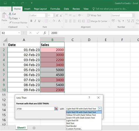
Identifying Sales Trends: In a sales dataset, you could use conditional formatting to highlight rows where sales exceeded a certain threshold or where there was a significant increase from the previous period.
Flagging Errors: Conditional formatting can be used to highlight rows where data validation checks fail, indicating potential errors or inconsistencies in the data.

Advanced Conditional Formatting Techniques

For more complex scenarios, Google Sheets supports the use of custom formulas in conditional formatting. This allows for very specific and sophisticated formatting rules. For example, you might use a formula that checks multiple conditions or refers to values in other cells or sheets.

Best Practices for Conditional Formatting

To get the most out of conditional formatting and ensure your spreadsheets remain organized and easy to understand, follow these best practices:

Keep it Simple: Avoid overly complex formatting rules that might be hard to understand or maintain.
Use Consistent Formatting: Apply consistent formatting throughout your spreadsheet to make it easier to read and understand.
Test Your Rules: Always test your conditional formatting rules to ensure they work as expected.

Gallery of Conditional Formatting Examples

Conditional Formatting Image Gallery

What is conditional formatting in Google Sheets?

Conditional formatting in Google Sheets is a feature that allows you to apply formatting to cells based on specific conditions, such as the cell's value, the cell's format, or custom formulas.

How do I apply conditional formatting to an entire row based on a cell's value?

To apply conditional formatting to an entire row based on a cell's value, select the range of cells, go to the "Format" tab, select "Conditional formatting," and then use a custom formula that refers to the cell you want to base the formatting on.

What are some common use cases for conditional row formatting?

Common use cases include highlighting priority tasks, identifying sales trends, and flagging errors in data. Conditional formatting can be used in any scenario where visual distinction based on cell values is beneficial.

In conclusion, conditional formatting is a powerful tool in Google Sheets that can greatly enhance the usability and readability of your spreadsheets. By applying formatting rules based on cell values, you can draw attention to important information, identify trends, and make your data more intuitive. Whether you're managing tasks, analyzing sales data, or simply organizing information, conditional formatting can help you get more out of your spreadsheets. So, explore the possibilities of conditional formatting, and discover how it can transform your workflow and decision-making processes.