Intro
Inserting multiple pivot tables in a single Excel sheet can be a powerful way to analyze and visualize data from different perspectives. Pivot tables are a crucial tool in data analysis, allowing users to summarize, analyze, and present large datasets in a meaningful way. When you have multiple pivot tables in one sheet, it enables comparisons and insights that might not be immediately apparent from a single table. Here's a step-by-step guide on how to insert two pivot tables in one sheet, along with tips on managing and customizing them for better data analysis.
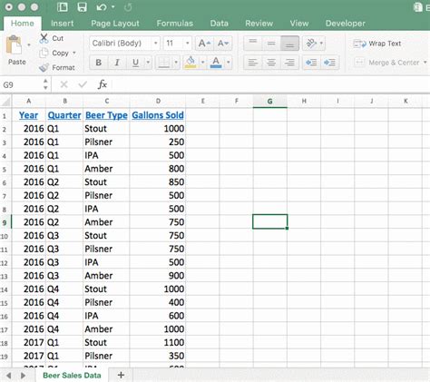
To start, ensure you have a dataset ready. This could be sales data, customer information, or any other type of data you wish to analyze. For this example, let's assume we're working with sales data that includes columns for date, region, product, and sales amount.
Preparing Your Data
Before creating pivot tables, your data should be organized in a table format with headers in the first row. Each column should represent a field (e.g., date, region, product), and each row should represent a single record or entry. Ensure there are no blank rows or columns within your data range, as this can cause issues when creating pivot tables.
Creating the First Pivot Table
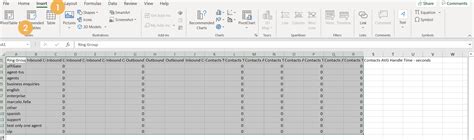
- Select any cell within your data range.
- Go to the "Insert" tab on the ribbon.
- Click on "PivotTable." This will open the "Create PivotTable" dialog box.
- Choose a cell where you want the pivot table to be placed. You can place it in a new worksheet or in an existing one. For this example, we'll place it in the existing sheet.
- Click "OK" to create the pivot table.
Customizing the First Pivot Table
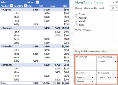
- Drag the "Region" field to the "Row Labels" area to see sales by region.
- Drag the "Product" field to the "Column Labels" area to compare sales across different products.
- Drag the "Sales Amount" field to the "Values" area to quantify the sales.
This setup will give you a pivot table that shows sales amounts by region and product, allowing for a detailed comparison across these dimensions.
Creating the Second Pivot Table

To insert a second pivot table, follow the same steps as before, but this time, choose a different cell for the pivot table to be placed, ensuring it doesn't overlap with the first pivot table.
Customizing the Second Pivot Table
For the second pivot table, you might want to analyze sales by date and product. So, you would:
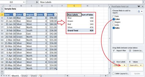
- Drag the "Date" field to the "Row Labels" area.
- Drag the "Product" field to the "Column Labels" area.
- Drag the "Sales Amount" field to the "Values" area.
This setup will provide a view of sales over time for each product, which can be useful for identifying trends or seasonal patterns.
Managing Multiple Pivot Tables
Managing multiple pivot tables in one sheet requires some planning to ensure clarity and ease of use. Here are some tips:
- Use Clear Headers: Ensure each pivot table has a clear and descriptive header that indicates what it represents.
- Organize Tables: Place related pivot tables close to each other to facilitate comparison.
- Synchronize Filters: If you have common fields across pivot tables (like "Product"), you can synchronize filters so that selecting a filter in one pivot table automatically applies to the others.
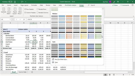
- Use Pivot Table Tools: The "PivotTable Tools" tab on the ribbon provides various options for customizing the appearance and behavior of your pivot tables.
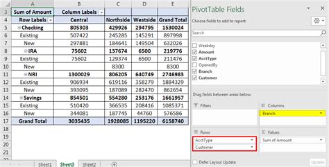
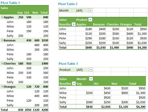
Gallery of Pivot Table Examples
Pivot Table Image Gallery


Frequently Asked Questions
How do I update my pivot table after changing my data?
+To update your pivot table, simply right-click on the pivot table and select "Refresh" or use the "Refresh All" button in the "Data" tab if you have multiple pivot tables and data connections.
Can I have multiple pivot tables based on the same data source?
+Yes, you can have multiple pivot tables based on the same data source. This is useful for analyzing the data from different perspectives without having to duplicate the data.
How do I change the data source of an existing pivot table?
+To change the data source, go to the "PivotTable Tools" tab, click on "Options," then "Change Data Source," and select the new range or table you want to use.
Inserting two pivot tables in one sheet is a straightforward process that can significantly enhance your data analysis capabilities. By customizing each pivot table to focus on different aspects of your data, you can gain a more comprehensive understanding of your dataset. Remember to keep your pivot tables organized, use clear and descriptive headers, and take advantage of Excel's tools to manage and customize your pivot tables for the best results. If you have any further questions or need more detailed guidance on specific steps, feel free to ask in the comments below.