Index Match Multiple Criteria Google Sheets

The INDEX-MATCH function combination in Google Sheets is a powerful tool for looking up and retrieving data from a table based on one or more criteria. When you need to match multiple criteria, this function becomes even more versatile, allowing you to perform complex lookups with ease. In this article, we'll delve into how to use the INDEX-MATCH function to match multiple criteria in Google Sheets, exploring its benefits, working mechanisms, and providing practical examples to enhance your understanding.

The importance of being able to look up data based on multiple criteria cannot be overstated, especially in data analysis and management. Whether you're dealing with sales data, inventory management, or any other type of dataset, the ability to filter and retrieve specific information quickly is crucial for making informed decisions. The INDEX-MATCH function offers a flexible and efficient way to achieve this, making it a valuable skill for anyone working with data in Google Sheets.

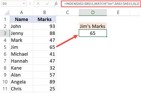
Before we dive into the specifics of using INDEX-MATCH for multiple criteria, it's essential to understand the basic components of this function combination. The INDEX function returns a value at a specified position in a range or array, while the MATCH function returns the position of a value within a range. When combined, they enable you to look up a value in a table and return a corresponding value from another column. This basic functionality can then be expanded to accommodate multiple lookup criteria.

Understanding the INDEX-MATCH Function

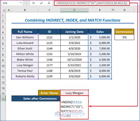
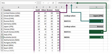
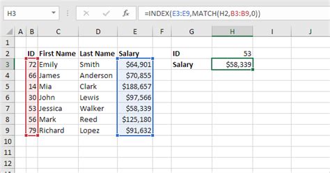
To use the INDEX-MATCH function for matching multiple criteria, you typically follow a structured approach. First, you need to understand your data layout and identify the columns that contain your lookup criteria and the column from which you want to retrieve the data. The general syntax for the INDEX-MATCH function when matching a single criterion is INDEX(range, MATCH(lookup_value, lookup_range, [match_type]), where range is the range from which to return a value, lookup_value is the value you want to look up, lookup_range is the range where lookup_value should be searched, and [match_type] specifies whether you want an exact match or an approximate match.

Expanding to Multiple Criteria

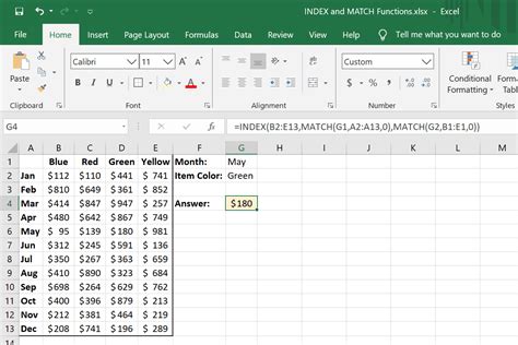
When you need to match multiple criteria, you can use the INDEX-MATCH combination in conjunction with the & operator, which acts as a logical AND operator in Google Sheets formulas. This means that your lookup will only return values that match all specified criteria. The formula structure expands to include multiple MATCH functions, each looking up a different criterion, and these are combined using the & operator.

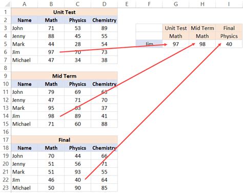
For example, if you have a table with names, ages, and cities, and you want to find the age of a person named "John" who lives in "New York", your formula might look something like this: =INDEX(C:C, MATCH(1, (A:A="John") * (B:B="New York"), 0)), assuming names are in column A, cities in column B, and ages in column C. This formula uses the MATCH function to find the row where both conditions ("John" and "New York") are true and then uses INDEX to return the age from that row.

Practical Examples and Applications

Let's consider a more detailed example to illustrate the power and flexibility of the INDEX-MATCH function with multiple criteria. Suppose you have a sales dataset that includes columns for the salesperson's name, region, product, and sales amount. You want to find the total sales amount for a specific salesperson in a particular region for a certain product.

1. Setup Your Data: Ensure your data is organized in a table format with clear headers.
2. Identify Your Criteria: Determine what you're looking for, such as the salesperson's name, region, and product.
3. Construct Your Formula: Use the INDEX-MATCH function combination, incorporating the & operator to match multiple criteria. For instance, =INDEX(D:D, MATCH(1, (A:A="Salesperson Name") * (B:B="Region") * (C:C="Product"), 0)), where D:D contains the sales amounts.

Tips and Variations

• Using Multiple Criteria with Different Operators: You can combine the & (AND) operator with the + (OR) operator in your lookup criteria by using parentheses to specify the order of operations.
• Handling Errors: Use the IFERROR function to handle cases where no match is found, providing a default value or message instead of an error.
• Dynamic Lookups: Incorporate cell references into your lookup criteria to make your formulas dynamic and responsive to changes in your worksheet.

Advanced Applications and Best Practices

As you become more comfortable with the INDEX-MATCH function, you can explore more advanced applications, such as using arrays to perform lookups across multiple tables or incorporating other Google Sheets functions to enhance your data analysis capabilities.

• Array Formulas: Use the INDEX-MATCH combination within array formulas to perform complex lookups and calculations across your dataset.
• Data Validation: Combine INDEX-MATCH with data validation to create dropdown menus that update based on user selections, enhancing the user experience and reducing errors.

Conclusion and Next Steps

Mastering the INDEX-MATCH function for matching multiple criteria in Google Sheets opens up a world of possibilities for data analysis and management. By following the examples and tips provided in this article, you'll be well on your way to becoming proficient in using this powerful function combination. Remember to practice regularly and explore the many resources available online to deepen your understanding of Google Sheets and its capabilities.

Gallery of INDEX-MATCH Examples

INDEX-MATCH Function Gallery

What is the INDEX-MATCH function used for in Google Sheets?

+

The INDEX-MATCH function combination is used for looking up and retrieving data from a table based on one or more criteria, offering a flexible and efficient way to perform complex data lookups.

How do I use the INDEX-MATCH function to match multiple criteria?

+

To match multiple criteria, use the `&` operator to combine multiple `MATCH` functions, each looking up a different criterion. The general syntax is `INDEX(range, MATCH(1, (criteria1) * (criteria2) *..., 0))`.

What are some common challenges when using the INDEX-MATCH function?

+

Common challenges include handling errors when no match is found, using the correct match type, and ensuring that the lookup range and return range are correctly specified.

We hope this comprehensive guide to using the INDEX-MATCH function for matching multiple criteria in Google Sheets has been informative and helpful. Whether you're a beginner looking to enhance your data analysis skills or an advanced user seeking to optimize your workflows, mastering this function combination can significantly improve your productivity and efficiency. Don't hesitate to share your thoughts, ask questions, or provide feedback in the comments below. Your input is invaluable in helping us create more relevant and useful content for our readers.