Rank In Excel By Multiple Criteria

Ranking data in Excel by multiple criteria is a common task that can help you analyze and understand your data better. Whether you're dealing with sales data, student grades, or any other type of data, being able to rank it based on multiple conditions can provide valuable insights. In this article, we'll explore how to rank data in Excel by multiple criteria, including using formulas, pivot tables, and other methods.

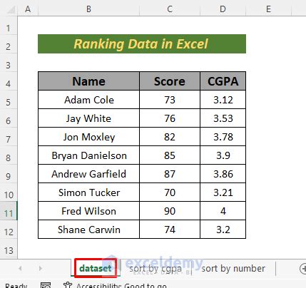
To start with, let's consider a simple example. Suppose you have a list of students with their names, ages, and test scores. You want to rank these students based on their test scores and then by their ages. This means that students with higher test scores should be ranked higher, and if two students have the same test score, the younger student should be ranked higher.

Using Formulas to Rank Data

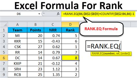
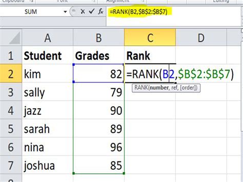
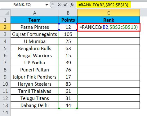
One way to rank data by multiple criteria in Excel is by using formulas. The most common formula used for ranking is the RANK function, which can rank numbers in a list in order from largest to smallest. However, when you need to rank by multiple criteria, you might need to combine the RANK function with other functions like IF or INDEX/MATCH.

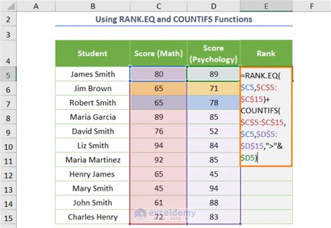
For example, if you have your data in columns A (Name), B (Age), and C (Test Score), and you want to rank the students first by Test Score and then by Age, you could use a formula like this:

=RANK(C2, C:C, 0) & "/" & COUNTIF(C:C, C2)

However, this formula only ranks by one criterion (Test Score) and doesn't account for the age. To rank by multiple criteria, you might need a more complex formula or an array formula, which can be cumbersome and not very flexible.

Using Pivot Tables for Ranking

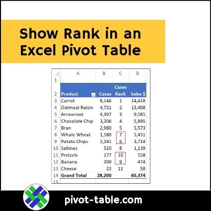
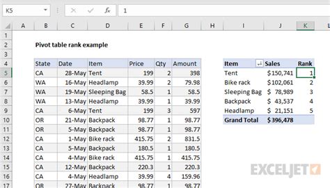
Pivot tables are another powerful tool in Excel for data analysis, including ranking data by multiple criteria. By using the "Rank" function within a pivot table, you can easily rank your data based on multiple fields.

To create a pivot table and rank your data:

Select your data range.
Go to the "Insert" tab and click on "PivotTable."
Choose a cell to place your pivot table and click "OK."
Drag the field you want to rank by (e.g., Test Score) to the "Values" area.
Right-click on the field in the "Values" area and select "Value Field Settings."
In the "Value Field Settings" dialog, click on the "Show value as" tab and select "Rank Largest to Smallest" or "Rank Smallest to Largest" depending on your needs.

To rank by multiple criteria, you can add another field to the "Row Labels" area and then use the "Rank" function in combination with this field.

Using Power Query for Advanced Ranking

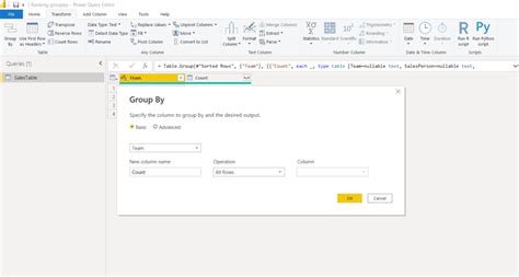
For more advanced ranking scenarios, especially when dealing with large datasets or complex ranking rules, Power Query (available in Excel 2013 and later versions) can be a very powerful tool. Power Query allows you to manipulate and analyze data from various sources, including tables within Excel.

To use Power Query for ranking:

Select your data range.
Go to the "Data" tab and click on "From Table/Range" in the "Get & Transform Data" group.
This opens Power Query Editor where you can add a custom column to rank your data.
Use the "Add Column" tab to add a new column, and then use the "Rank" function within the formula section to create your ranking logic.

The advantage of using Power Query is its flexibility and the ability to handle complex data transformations and ranking rules without the need for complex formulas.

Steps for Ranking in Power Query

Here are the general steps for ranking data in Power Query: - Load your data into Power Query. - Add a new column using the "Add Column" tab. - Use the `Rank` function or other relevant functions like `List.Rank` to create your ranking formula. - Adjust the ranking order as needed (e.g., ascending or descending). - Load your transformed data back into Excel.

Ranking with Conditional Formatting

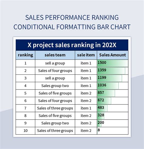
While not a direct method of ranking, conditional formatting can be used to highlight top or bottom values in your dataset based on multiple criteria. This can be particularly useful for visual analysis and reporting.

To apply conditional formatting for ranking:

Select your data range.
Go to the "Home" tab and click on "Conditional Formatting" in the "Styles" group.
Select "New Rule" and choose "Use a formula to determine which cells to format."
Enter a formula that identifies the top or bottom values based on your criteria (e.g., =RANK(C2, C:C, 0)<=10 for the top 10).
Format the cells as desired (e.g., fill color, font color).

Gallery of Ranking Examples

Ranking in Excel Gallery

Frequently Asked Questions

How do I rank data in Excel by multiple criteria?

You can rank data in Excel by multiple criteria using formulas, pivot tables, or Power Query. The method you choose depends on the complexity of your data and your specific ranking needs.

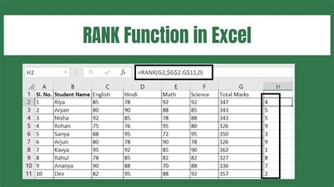
What is the RANK function in Excel, and how does it work?

The RANK function in Excel returns the rank of a number within a list of numbers. The syntax is RANK(number, ref, [order]), where "number" is the number to rank, "ref" is the list of numbers, and "[order]" specifies the ranking order (ascending or descending).

How can I use Power Query to rank data in Excel?

Power Query allows you to add a custom column to rank your data. You can use the "Rank" function within the formula section to create your ranking logic based on one or more criteria.

Can I use conditional formatting to highlight ranked data in Excel?

Yes, you can use conditional formatting to highlight top or bottom values in your dataset based on one or more criteria. This is useful for visual analysis and reporting.

What are the advantages of using pivot tables for ranking data in Excel?

Pivot tables offer a flexible way to rank data based on multiple fields. They also allow for easy filtering and grouping, making them a powerful tool for data analysis.

In conclusion, ranking data by multiple criteria in Excel is a versatile task that can be accomplished through various methods, including formulas, pivot tables, Power Query, and conditional formatting. Each method has its own advantages and is suited for different types of data analysis needs. By mastering these techniques, you can enhance your data analysis skills and make more informed decisions based on your data. Whether you're a beginner or an advanced Excel user, understanding how to rank data effectively can significantly improve your productivity and insights. So, take the time to explore these methods in more detail, and don't hesitate to reach out if you have any further questions or need additional guidance. Share your experiences with ranking data in Excel in the comments below, and feel free to share this article with others who might find it helpful.