5 Ways Vlookup

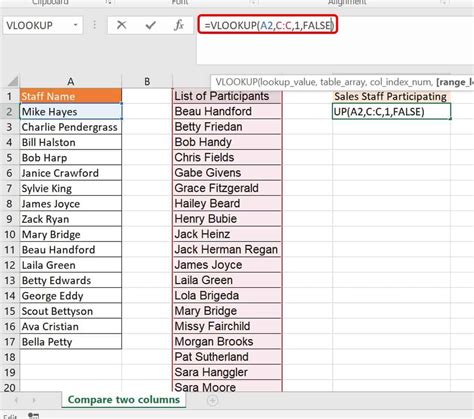
The Vlookup function is one of the most powerful and versatile tools in Microsoft Excel, allowing users to search for and retrieve data from a table or range by looking up a value in the first column. This function has numerous applications, from simple data retrieval to complex data analysis. In this article, we will explore five ways to use the Vlookup function, including its basic application, using it with multiple criteria, handling errors, and more.

The importance of understanding how to use the Vlookup function effectively cannot be overstated. It enables users to automate tasks, reduce manual data entry, and increase productivity. Moreover, it is a fundamental skill required in many professional settings, particularly in fields like finance, accounting, and data analysis. Whether you are a beginner looking to learn the basics of Excel or an advanced user seeking to expand your skill set, mastering the Vlookup function is essential.

For those who are new to Excel or need a refresher, the Vlookup function is used to look up a value in a table and return a value from another column. It is often used to retrieve data from large datasets, merge data from different sources, and perform data validation. The function is highly flexible and can be adapted to a wide range of scenarios, making it an indispensable tool for anyone working with data in Excel.

Basic Application of Vlookup

The basic application of the Vlookup function involves searching for a value in the first column of a table and returning a corresponding value from another column. The syntax for the Vlookup function is VLOOKUP(lookup_value, table_array, col_index_num, [range_lookup]). The lookup_value is the value you want to search for, the table_array is the range of cells that contains the data you want to search, the col_index_num is the column number that contains the value you want to return, and the [range_lookup] is an optional argument that specifies whether you want an exact or approximate match.

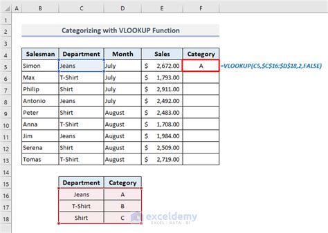
To illustrate this, let's consider an example. Suppose you have a table with employee names in the first column and their corresponding employee IDs in the second column. You can use the Vlookup function to retrieve an employee's ID by looking up their name. For instance, if the table is in the range A1:B10 and you want to find the ID of an employee named "John Doe", you would use the formula =VLOOKUP("John Doe", A1:B10, 2, FALSE).

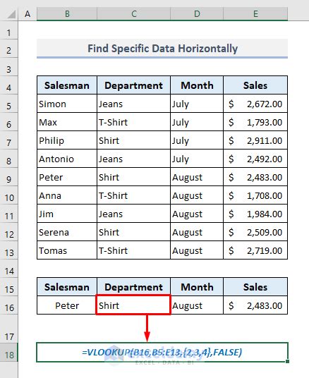
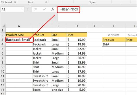
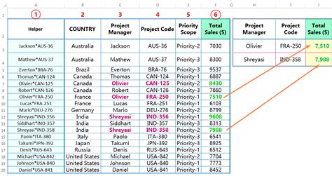
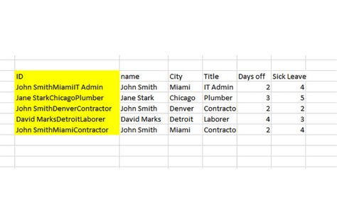
Using Vlookup with Multiple Criteria

In many cases, you may need to look up a value based on multiple criteria. While the Vlookup function itself does not support multiple lookup criteria, you can use it in conjunction with other functions, such as the INDEX and MATCH functions, to achieve this. One way to do this is by using an array formula that combines the INDEX and MATCH functions. For example, if you have a table with employee names in the first column, departments in the second column, and employee IDs in the third column, and you want to find the ID of an employee named "John Doe" in the "Sales" department, you can use an array formula like =INDEX(C:C, MATCH(1, (A:A="John Doe") * (B:B="Sales"), 0)).

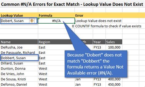
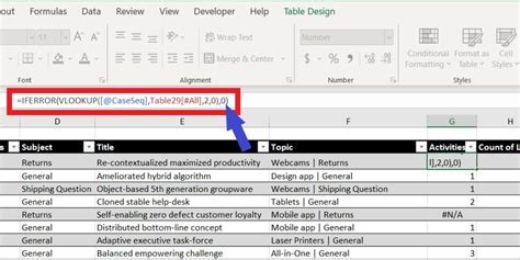
Handling Errors with Vlookup

One of the common issues with using the Vlookup function is handling errors. If the lookup value is not found in the table, the Vlookup function returns a #N/A error. To handle this, you can use the IFERROR function, which returns a custom value if the formula returns an error. For example, if you want to return a message like "Employee not found" instead of the #N/A error, you can use the formula =IFERROR(VLOOKUP("John Doe", A1:B10, 2, FALSE), "Employee not found").

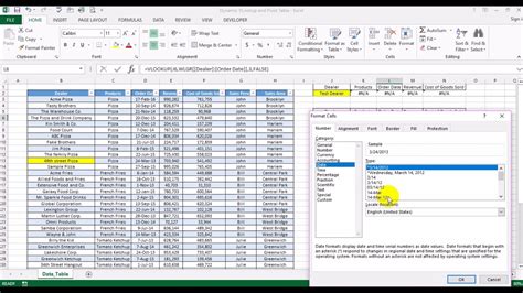
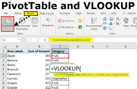
Using Vlookup with PivotTables

PivotTables are another powerful tool in Excel that can be used to summarize and analyze large datasets. You can use the Vlookup function in conjunction with PivotTables to retrieve data from a PivotTable based on a lookup value. For instance, if you have a PivotTable that summarizes sales data by region and product, and you want to find the total sales for a specific product in a specific region, you can use the Vlookup function to retrieve this data from the PivotTable.

Best Practices for Using Vlookup

To get the most out of the Vlookup function, there are several best practices you should follow. First, make sure the lookup value is in the first column of the table. Second, use absolute references for the table range to ensure the formula works correctly even if you insert or delete columns. Third, use the FALSE argument for the [range_lookup] to ensure an exact match. Finally, test your formula thoroughly to ensure it returns the correct results.

Gallery of Vlookup Examples

Vlookup Image Gallery

What is the Vlookup function used for?

+

The Vlookup function is used to search for a value in a table and return a corresponding value from another column.

How do I handle errors with the Vlookup function?

+

You can handle errors with the Vlookup function by using the IFERROR function, which returns a custom value if the formula returns an error.

Can I use the Vlookup function with multiple criteria?

+

Yes, you can use the Vlookup function with multiple criteria by combining it with other functions, such as the INDEX and MATCH functions.

What are some best practices for using the Vlookup function?

+

Some best practices for using the Vlookup function include making sure the lookup value is in the first column of the table, using absolute references for the table range, and testing your formula thoroughly.

How do I use the Vlookup function with PivotTables?

+

You can use the Vlookup function with PivotTables to retrieve data from a PivotTable based on a lookup value.

In conclusion, the Vlookup function is a powerful tool in Excel that can be used in a variety of ways to retrieve and analyze data. By mastering the Vlookup function, you can automate tasks, reduce manual data entry, and increase productivity. We hope this article has provided you with a comprehensive understanding of how to use the Vlookup function effectively. If you have any further questions or would like to share your own tips and tricks for using the Vlookup function, please don't hesitate to comment below. Additionally, if you found this article helpful, please share it with your friends and colleagues who may also benefit from learning about the Vlookup function.