Intro
Master Excels Vlookup function with 2 columns, using index-match, approximate matches, and multiple criteria to simplify data analysis and lookup tasks efficiently.
Looking for ways to use Vlookup with two columns can be a bit tricky, but it's a useful skill to have in Excel. The Vlookup function is a powerful tool that allows you to search for a value in a table and return a corresponding value from another column. While it's typically used to look up values in a single column, there are ways to adapt it to work with two columns. In this article, we'll explore five different methods to achieve this.
The importance of being able to Vlookup two columns lies in its ability to increase the accuracy and efficiency of your data analysis. By being able to look up values in multiple columns, you can reduce errors and improve the overall quality of your data. Whether you're working with large datasets or small ones, being able to Vlookup two columns is an essential skill for any Excel user.
One of the key benefits of using Vlookup with two columns is its ability to handle complex data sets. By being able to look up values in multiple columns, you can quickly and easily identify patterns and trends in your data. This can be especially useful when working with large datasets, where manual analysis can be time-consuming and prone to errors. With Vlookup, you can automate the process and get accurate results in a fraction of the time.
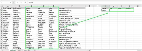
Method 1: Using the Vlookup Function with Two Columns
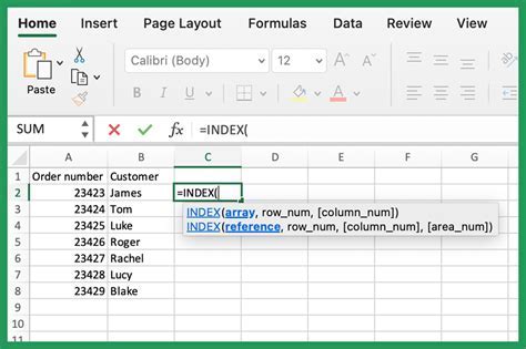
Method 2: Using the Index and Match Functions
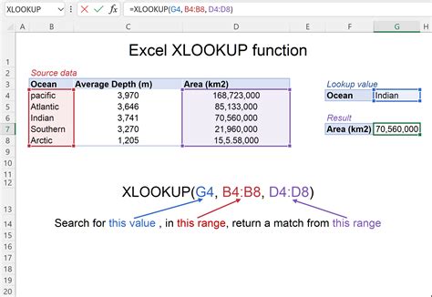
Method 3: Using the Xlookup Function
Method 4: Using the Filter Function

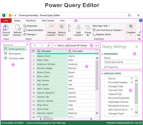
Method 5: Using the Power Query Editor
Gallery of Vlookup 2 Columns
Vlookup 2 Columns Image Gallery


What is the Vlookup function?
+The Vlookup function is a built-in Excel function that allows you to search for a value in a table and return a corresponding value from another column.
How do I use the Vlookup function with two columns?
+To use the Vlookup function with two columns, you can use the formula `=VLOOKUP(A2, B:C, 2, FALSE)`, where A2 is the value you want to look up, B:C is the range of cells that contains the data, and 2 is the column number that you want to return.
What is the Index and Match function?
+The Index and Match function is a combination of two Excel functions that allows you to look up a value in a table and return a corresponding value from another column. The formula for this function is `=INDEX(C:C, MATCH(A2, B:B, 0))`, where A2 is the value you want to look up, B:B is the range of cells that contains the data, and C:C is the range of cells that contains the values you want to return.
We hope this article has been helpful in showing you how to use the Vlookup function with two columns. Whether you're a beginner or an advanced user, being able to Vlookup two columns is an essential skill for any Excel user. By following the methods outlined in this article, you can improve your data analysis skills and become more efficient in your work. If you have any questions or need further assistance, please don't hesitate to comment below. We'd love to hear from you and help you with any Excel-related questions you may have.