Intro
Compare two columns in Excel easily with formulas and functions, using VLOOKUP, INDEX-MATCH, and conditional formatting to identify duplicates, differences, and similarities between data sets.
Comparing two columns in Excel is a common task that can help you identify duplicates, differences, or matches between two sets of data. Whether you're working with a small dataset or a large one, Excel provides several ways to compare columns, each with its own advantages and use cases. In this article, we'll delve into the various methods you can use to compare two columns in Excel, exploring their steps, benefits, and examples.
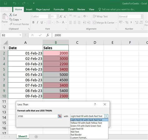
When comparing two columns, it's essential to understand what you're looking for. Are you trying to find duplicate values, identify unique entries, or highlight differences? Each of these objectives requires a slightly different approach. For instance, if you're looking to find duplicate values, using the Conditional Formatting feature can be highly effective. On the other hand, if your goal is to identify unique entries in one column that are not present in another, formulas like IF and VLOOKUP can be invaluable.
Using Conditional Formatting to Compare Columns
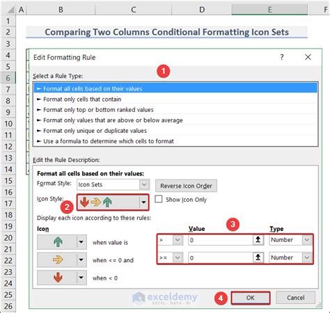
Conditional Formatting is a powerful tool in Excel that allows you to highlight cells based on specific conditions. To compare two columns using Conditional Formatting, you can follow these steps:
- Select the entire column you want to format.
- Go to the Home tab, find the Styles group, and click on Conditional Formatting.
- Choose "New Rule" and then select "Use a formula to determine which cells to format."
- Enter a formula that compares the two columns. For example, if you want to highlight duplicates between column A and column B, you could use a formula like
=COUNTIF(B:B, A1) > 0. - Click Format to choose how you want to highlight the cells, and then click OK.
Using Formulas to Compare Columns

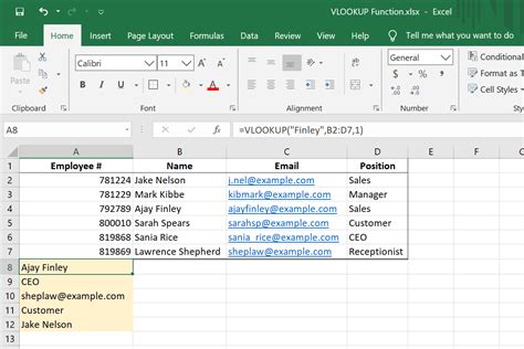
Formulas provide a flexible way to compare columns, allowing for a wide range of comparisons. For example, to find if a value in column A exists in column B, you can use the VLOOKUP function. The syntax for VLOOKUP is VLOOKUP(lookup_value, table_array, col_index_num, [range_lookup]). If you're looking to identify unique values in column A that are not in column B, you might use a formula like =IF(ISERROR(VLOOKUP(A1, B:B, 1, FALSE)), "Unique", "Duplicate").
Steps for Using VLOOKUP
To use VLOOKUP for comparing columns: 1. Decide on the lookup value (the cell you want to search for). 2. Choose the table array (the range of cells where you want to search). 3. Determine the column index number (the column in the table array that contains the value you want to return). 4. Optionally, specify if you want an exact match or an approximate match.Using PivotTables to Compare Columns
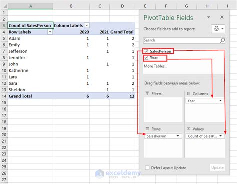
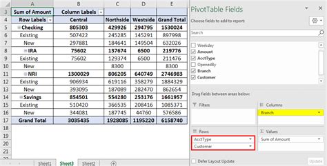
PivotTables are another powerful tool in Excel that can help you summarize and analyze large datasets. To compare two columns using a PivotTable, you can follow these steps:
- Select a cell where you want to place your PivotTable.
- Go to the Insert tab and click on PivotTable.
- Choose the table or range that contains your data.
- Drag one column to the Row Labels area and the other to the Column Labels area.
- Use the Values area to summarize the data, such as counting the occurrences of each combination.
Benefits of Using PivotTables
PivotTables offer several benefits for comparing columns, including the ability to easily summarize large datasets, filter data based on conditions, and create interactive dashboards.Using Power Query to Compare Columns
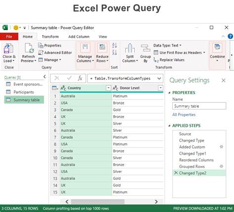
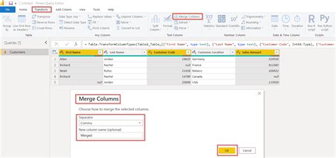
Power Query is a business intelligence tool in Excel that allows you to discover, combine, and refine data. To compare two columns using Power Query:
- Select the data range that includes the two columns you want to compare.
- Go to the Data tab and click on From Table/Range.
- In the Power Query Editor, you can use the Merge & Append group to compare or combine queries.
Steps for Merging Queries
To merge queries in Power Query: 1. Open the Power Query Editor. 2. Go to the Home tab and click on Merge Queries. 3. Select the queries you want to merge and the join kind (e.g., inner join, left outer join). 4. Choose the columns to match and click OK.Gallery of Comparison Methods
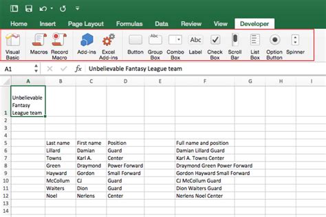
Comparison Methods Image Gallery


What is the easiest way to compare two columns in Excel?
+The easiest way often involves using Conditional Formatting for a quick visual comparison or the VLOOKUP function for more detailed analysis.
Can I compare columns from different worksheets or workbooks?
+Yes, you can compare columns from different worksheets or workbooks by referencing the specific range in your formula or by using Power Query to merge data from different sources.
How do I highlight duplicates between two columns?
+You can highlight duplicates by using Conditional Formatting with a formula that checks for the existence of a value in one column within another column.
In conclusion, comparing two columns in Excel is a versatile task that can be accomplished through various methods, each suited to different needs and preferences. Whether you're using Conditional Formatting for a quick glance, formulas for detailed analysis, PivotTables for summarization, or Power Query for advanced data manipulation, Excel offers a robust set of tools to help you compare and contrast your data effectively. By mastering these techniques, you can unlock deeper insights into your data, making more informed decisions in your personal or professional endeavors. Feel free to share your experiences or tips on comparing columns in Excel in the comments below, and don't hesitate to reach out if you have any further questions or need additional guidance on any of the methods discussed.