Intro
Discover how to Excel compare two lists for differences using formulas, VLOOKUP, and conditional formatting to identify mismatches, duplicates, and unique values.
When working with data in Excel, it's common to have two lists that you want to compare for differences. This can be useful in a variety of situations, such as identifying new customers, finding discrepancies in inventory, or highlighting changes in data over time. Fortunately, Excel provides several ways to compare two lists for differences, making it easy to analyze and understand your data.
The ability to compare two lists in Excel is a powerful tool that can help you make informed decisions, identify trends, and optimize your workflows. By using the methods outlined in this article, you'll be able to quickly and easily compare two lists and identify the differences between them. This can help you streamline your processes, improve accuracy, and reduce errors.
In today's fast-paced business environment, being able to quickly and easily compare data is crucial. By mastering the techniques outlined in this article, you'll be able to stay ahead of the curve and make data-driven decisions with confidence. Whether you're working with customer lists, inventory data, or financial information, the ability to compare two lists in Excel is an essential skill that can help you achieve your goals.
Using the IF Function to Compare Two Lists
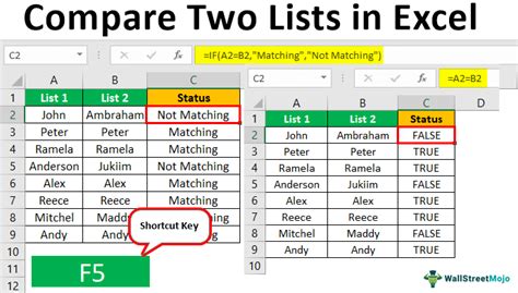
One way to compare two lists in Excel is by using the IF function. This function allows you to test a condition and return one value if the condition is true and another value if it's false. To use the IF function to compare two lists, you'll need to set up a formula that checks for the presence of each value in the first list within the second list.
For example, suppose you have two lists of customer IDs, one in column A and the other in column B. You can use the IF function to identify which customer IDs are present in column A but not in column B. The formula would look like this: =IF(ISERROR(MATCH(A2, B:B, 0)), "Not Found", "Found").
How to Use the IF Function to Compare Two Lists
To use the IF function to compare two lists, follow these steps: * Select the cell where you want to display the result * Type =IF(ISERROR(MATCH( * Select the cell containing the value you want to look up * Type, B:B, 0)), * Type "Not Found", "Found") * Press EnterUsing the VLOOKUP Function to Compare Two Lists
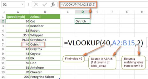
Another way to compare two lists in Excel is by using the VLOOKUP function. This function allows you to look up a value in a table and return a corresponding value from another column. To use the VLOOKUP function to compare two lists, you'll need to set up a formula that looks up each value in the first list within the second list.
For example, suppose you have two lists of customer names, one in column A and the other in column B. You can use the VLOOKUP function to identify which customer names are present in column A but not in column B. The formula would look like this: =VLOOKUP(A2, B:C, 2, FALSE).
How to Use the VLOOKUP Function to Compare Two Lists
To use the VLOOKUP function to compare two lists, follow these steps: * Select the cell where you want to display the result * Type =VLOOKUP( * Select the cell containing the value you want to look up * Type, B:C, 2, FALSE) * Press EnterUsing the INDEX/MATCH Function to Compare Two Lists
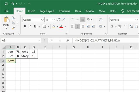
The INDEX/MATCH function is another way to compare two lists in Excel. This function allows you to look up a value in a table and return a corresponding value from another column. To use the INDEX/MATCH function to compare two lists, you'll need to set up a formula that looks up each value in the first list within the second list.
For example, suppose you have two lists of product codes, one in column A and the other in column B. You can use the INDEX/MATCH function to identify which product codes are present in column A but not in column B. The formula would look like this: =INDEX(C:C, MATCH(A2, B:B, 0)).
How to Use the INDEX/MATCH Function to Compare Two Lists
To use the INDEX/MATCH function to compare two lists, follow these steps: * Select the cell where you want to display the result * Type =INDEX( * Select the column containing the values you want to return * Type, MATCH( * Select the cell containing the value you want to look up * Type, B:B, 0)) * Press EnterUsing Conditional Formatting to Compare Two Lists
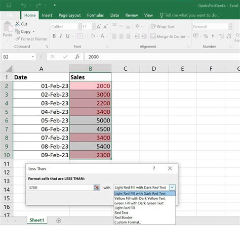
Conditional formatting is another way to compare two lists in Excel. This feature allows you to highlight cells based on specific conditions, such as the presence of a value in another list. To use conditional formatting to compare two lists, you'll need to select the cells you want to format and then apply a rule that checks for the presence of each value in the first list within the second list.
For example, suppose you have two lists of employee names, one in column A and the other in column B. You can use conditional formatting to highlight the employee names that are present in column A but not in column B.
How to Use Conditional Formatting to Compare Two Lists
To use conditional formatting to compare two lists, follow these steps: * Select the cells you want to format * Go to the Home tab * Click on Conditional Formatting * Select New Rule * Select Use a formula to determine which cells to format * Type =ISERROR(MATCH(A2, B:B, 0)) * Click Format * Select a fill color * Click OKExcel Compare Two Lists Image Gallery

What is the best way to compare two lists in Excel?
+The best way to compare two lists in Excel depends on your specific needs and the structure of your data. You can use the IF function, VLOOKUP function, INDEX/MATCH function, or conditional formatting to compare two lists.
How do I use the IF function to compare two lists?
+To use the IF function to compare two lists, you'll need to set up a formula that checks for the presence of each value in the first list within the second list. The formula would look like this: =IF(ISERROR(MATCH(A2, B:B, 0)), "Not Found", "Found").
What is the difference between the VLOOKUP and INDEX/MATCH functions?
+The VLOOKUP and INDEX/MATCH functions are both used to look up values in a table and return a corresponding value from another column. However, the VLOOKUP function is more straightforward and easier to use, while the INDEX/MATCH function is more flexible and powerful.
In summary, comparing two lists in Excel can be a powerful tool for analyzing and understanding your data. By using the IF function, VLOOKUP function, INDEX/MATCH function, or conditional formatting, you can quickly and easily identify the differences between two lists. Whether you're working with customer data, inventory data, or financial information, the ability to compare two lists in Excel is an essential skill that can help you make informed decisions and drive business success. We hope this article has provided you with the knowledge and skills you need to compare two lists in Excel with confidence. If you have any further questions or need additional assistance, please don't hesitate to reach out.