Intro
Learn Excel comparing multiple columns techniques, including VLOOKUP, INDEX-MATCH, and conditional formatting, to efficiently compare and analyze data across multiple columns and rows.
Comparing multiple columns in Excel can be a daunting task, especially when dealing with large datasets. However, Excel provides various tools and functions to make this process easier and more efficient. In this article, we will explore the different methods for comparing multiple columns in Excel, including using formulas, conditional formatting, and pivot tables.
When working with multiple columns, it's essential to understand the importance of data analysis and comparison. By comparing multiple columns, you can identify trends, patterns, and relationships between different data points. This can help you make informed decisions, optimize processes, and improve overall performance. Whether you're working with sales data, customer information, or financial records, comparing multiple columns is a crucial step in extracting valuable insights from your data.
Comparing multiple columns can be used in various scenarios, such as identifying duplicate records, finding mismatched data, or highlighting differences between different datasets. For instance, in a sales database, you might want to compare the sales figures of different products, regions, or time periods to identify areas of growth or decline. By using the right tools and techniques, you can quickly and easily compare multiple columns and gain a deeper understanding of your data.
Using Formulas to Compare Multiple Columns
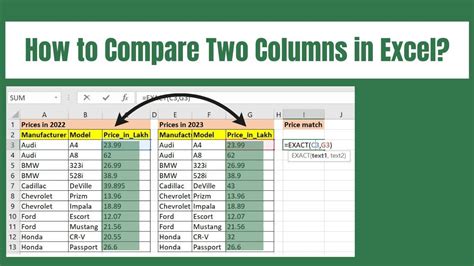
One of the most common methods for comparing multiple columns in Excel is by using formulas. You can use the IF function, the IFERROR function, or the VLOOKUP function to compare values between different columns. For example, if you want to compare the values in column A and column B, you can use the formula: =IF(A1=B1, "Match", "No Match"). This formula will return "Match" if the values in cell A1 and cell B1 are the same, and "No Match" if they are different.
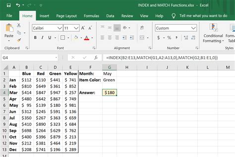
Another way to compare multiple columns using formulas is by using the INDEX and MATCH functions. These functions allow you to look up values in a table and return a corresponding value from another column. For example, if you want to compare the values in column A and column C, you can use the formula: =INDEX(C:C, MATCH(A1, A:A, 0)). This formula will return the value in column C that corresponds to the value in cell A1.
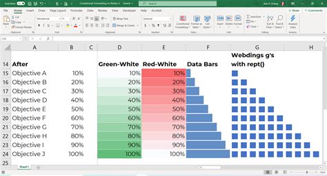
Using Conditional Formatting to Compare Multiple Columns
Conditional formatting is another useful tool for comparing multiple columns in Excel. You can use conditional formatting to highlight cells that contain duplicate values, mismatched data, or values that meet certain criteria. For example, if you want to highlight cells in column A that contain the same value as cells in column B, you can use the formula: =A1=B1. This formula will highlight cells in column A that contain the same value as cells in column B.You can also use conditional formatting to compare multiple columns and highlight cells that contain values that meet certain criteria. For example, if you want to highlight cells in column A that contain values greater than the values in column B, you can use the formula: =A1>B1. This formula will highlight cells in column A that contain values greater than the values in column B.
Using Pivot Tables to Compare Multiple Columns
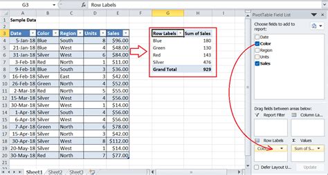
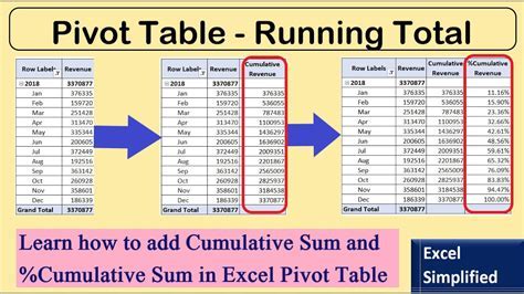
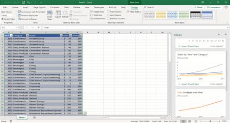
Pivot tables are a powerful tool for comparing multiple columns in Excel. You can use pivot tables to summarize and analyze large datasets, and to compare values between different columns. For example, if you want to compare the sales figures of different products, you can create a pivot table that summarizes the sales data by product.
To create a pivot table, you can select the data range that you want to analyze, and then go to the "Insert" tab in the ribbon. Click on the "PivotTable" button, and then select a cell where you want to place the pivot table. You can then drag the fields that you want to analyze to the "Row Labels" and "Column Labels" areas, and select the values that you want to summarize.
Using the VLOOKUP Function to Compare Multiple Columns
The VLOOKUP function is a useful tool for comparing multiple columns in Excel. You can use the VLOOKUP function to look up values in a table and return a corresponding value from another column. For example, if you want to compare the values in column A and column C, you can use the formula: =VLOOKUP(A1, A:C, 3, FALSE). This formula will return the value in column C that corresponds to the value in cell A1.You can also use the VLOOKUP function to compare multiple columns and return multiple values. For example, if you want to compare the values in column A and column C, and return the values in columns C and D, you can use the formula: =VLOOKUP(A1, A:D, {3,4}, FALSE). This formula will return the values in columns C and D that correspond to the value in cell A1.
Using the INDEX and MATCH Functions to Compare Multiple Columns

The INDEX and MATCH functions are useful tools for comparing multiple columns in Excel. You can use the INDEX and MATCH functions to look up values in a table and return a corresponding value from another column. For example, if you want to compare the values in column A and column C, you can use the formula: =INDEX(C:C, MATCH(A1, A:A, 0)). This formula will return the value in column C that corresponds to the value in cell A1.
You can also use the INDEX and MATCH functions to compare multiple columns and return multiple values. For example, if you want to compare the values in column A and column C, and return the values in columns C and D, you can use the formula: =INDEX(C:D, MATCH(A1, A:A, 0), {1,2}). This formula will return the values in columns C and D that correspond to the value in cell A1.
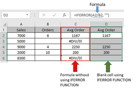
Using the IFERROR Function to Compare Multiple Columns
The IFERROR function is a useful tool for comparing multiple columns in Excel. You can use the IFERROR function to return a custom value if an error occurs when comparing values between different columns. For example, if you want to compare the values in column A and column B, and return a custom value if the values are not the same, you can use the formula: =IFERROR(A1/B1, "Error"). This formula will return the result of the division if the values are the same, and the custom value "Error" if the values are not the same.You can also use the IFERROR function to compare multiple columns and return multiple values. For example, if you want to compare the values in column A and column C, and return the values in columns C and D if the values are the same, you can use the formula: =IFERROR(INDEX(C:D, MATCH(A1, A:A, 0)), "Error"). This formula will return the values in columns C and D if the values are the same, and the custom value "Error" if the values are not the same.
Gallery of Excel Comparing Multiple Columns
Excel Comparing Multiple Columns Image Gallery


What is the best way to compare multiple columns in Excel?
+The best way to compare multiple columns in Excel depends on the specific task and data. You can use formulas, conditional formatting, pivot tables, or a combination of these methods to compare multiple columns.
How do I use the VLOOKUP function to compare multiple columns?
+The VLOOKUP function can be used to look up values in a table and return a corresponding value from another column. You can use the formula: =VLOOKUP(A1, A:C, 3, FALSE) to compare the values in column A and column C.
What is the difference between the INDEX and MATCH functions?
+The INDEX and MATCH functions are both used to look up values in a table and return a corresponding value from another column. However, the INDEX function returns a value based on its position in a range, while the MATCH function returns the relative position of a value within a range.
How do I use conditional formatting to compare multiple columns?
+Conditional formatting can be used to highlight cells that contain duplicate values, mismatched data, or values that meet certain criteria. You can use the formula: =A1=B1 to highlight cells in column A that contain the same value as cells in column B.
What is the best way to analyze and visualize data in Excel?
+The best way to analyze and visualize data in Excel depends on the specific task and data. You can use pivot tables, charts, and conditional formatting to analyze and visualize data. You can also use add-ins and third-party tools to enhance your data analysis and visualization capabilities.
In conclusion, comparing multiple columns in Excel can be a complex task, but there are various tools and functions that can make it easier and more efficient. By using formulas, conditional formatting, pivot tables, and other methods, you can quickly and easily compare multiple columns and gain a deeper understanding of your data. Whether you're working with sales data, customer information, or financial records, comparing multiple columns is a crucial step in extracting valuable insights from your data. We hope this article has provided you with the knowledge and skills to compare multiple columns in Excel and take your data analysis to the next level. If you have any questions or need further assistance, please don't hesitate to comment below. Share this article with your friends and colleagues to help them improve their Excel skills and data analysis capabilities.