Excel Conditional Formatting Older Dates

Conditional formatting in Excel is a powerful tool that allows users to highlight cells based on specific conditions, making it easier to visualize and analyze data. One common use of conditional formatting is to highlight older dates in a dataset. This can be particularly useful in managing tasks, tracking deadlines, or analyzing historical data. In this article, we will explore how to use Excel's conditional formatting feature to highlight older dates, providing step-by-step guides, examples, and tips to enhance your Excel skills.

Excel conditional formatting offers a range of options, including formatting cells based on their values, formulas, or even the format of the cells themselves. When it comes to dates, Excel treats them as serial numbers, where each date corresponds to a unique number. This allows for easy comparison and calculation with dates. To highlight older dates, we can use formulas within the conditional formatting rules to compare dates against a specific criterion, such as today's date or a fixed date in the past.

Understanding Conditional Formatting

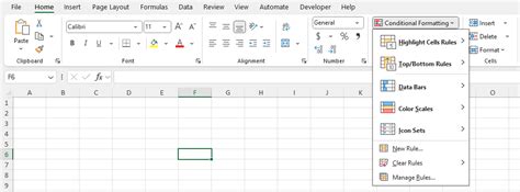
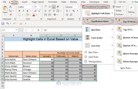
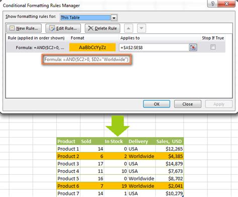
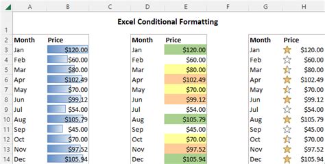
Conditional formatting in Excel can be accessed through the Home tab on the ribbon. The "Conditional Formatting" button in the Styles group offers several pre-set rules, including highlighting cells rules, top/bottom rules, data bars, color scales, and icon sets. For highlighting older dates, we typically use the "New Rule" option, which allows us to create a custom rule based on a formula.

Highlighting Older Dates

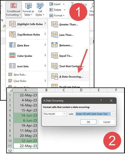
To highlight dates older than today, follow these steps:

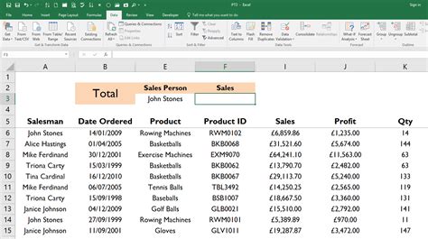
1. Select the range of cells that contain the dates you want to format.
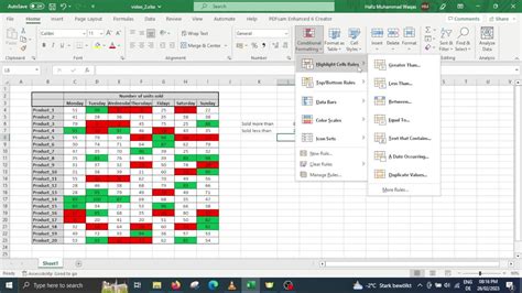
2. Go to the Home tab and click on "Conditional Formatting" in the Styles group.
3. Choose "New Rule" from the dropdown menu.
4. Select "Use a formula to determine which cells to format."
5. In the formula bar, enter a formula like =A1<TODAY(), assuming the date you want to check is in cell A1. This formula checks if the date in A1 is before today's date.
6. Click on the "Format" button to choose how you want to highlight the cells (e.g., fill color, font color).
7. Click OK to apply the rule.

Using Different Criteria

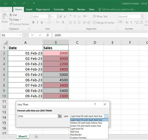
Sometimes, you might want to highlight dates based on different criteria, such as dates older than a specific number of days or dates within a certain range. Excel's conditional formatting is versatile and can accommodate these needs:

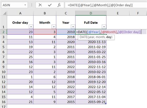
• To highlight dates older than 30 days, you can use a formula like =A1<TODAY()-30.
• To highlight dates within a specific range (e.g., between 1st January 2022 and 31st December 2022), you can use =AND(A1>DATE(2022,1,1), A1<DATE(2022,12,31)).

Applying Multiple Rules

Excel allows you to apply multiple conditional formatting rules to the same range of cells. This can be useful if you want to highlight dates based on multiple conditions, such as highlighting dates older than 30 days in one color and dates older than 60 days in another. To apply multiple rules:

1. Apply the first rule as described above.
2. Go back to the "Conditional Formatting" menu and select "New Rule" again.
3. Create your second rule, ensuring it applies to the same range of cells.
4. You can manage the order of your rules and decide whether to stop evaluating further rules once a cell has been formatted by using the "Manage Rules" option.

Tips and Variations

• Relative References: When creating formulas for conditional formatting, use relative references (e.g., A1) instead of absolute references (e.g., $A$1) so that the formula applies correctly to each cell in the selected range.
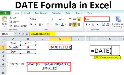
• Date Functions: Excel has a variety of date functions (e.g., TODAY(), DATE(), EOMONTH()) that can be used in conditional formatting formulas to create more complex rules.
• Format Priority: If multiple rules apply to the same cell, the rule that is applied last will override previous rules. Use the "Manage Rules" dialog to adjust the priority of your rules.

Conclusion and Next Steps

Mastering the art of conditional formatting in Excel can significantly enhance your data analysis and presentation skills. By applying the techniques outlined in this article, you can efficiently highlight older dates and other critical information in your datasets. Remember to experiment with different formulas and formatting options to tailor conditional formatting to your specific needs. Whether you're a beginner or an advanced Excel user, continuous practice and exploration of Excel's features will help you unlock more of its potential.

Excel Conditional Formatting Gallery

What is conditional formatting in Excel?

+

Conditional formatting is a feature in Excel that allows cells to be highlighted based on specific conditions, such as values, formulas, or cell formats.

How do I highlight older dates in Excel using conditional formatting?

+

To highlight older dates, select the date range, go to Conditional Formatting, choose New Rule, and use a formula like =A1

Can I apply multiple conditional formatting rules to the same range of cells?

+

Yes, Excel allows you to apply multiple rules. Use the Manage Rules option to adjust the priority of your rules if necessary.

We hope this comprehensive guide to highlighting older dates in Excel using conditional formatting has been informative and helpful. Whether you're managing projects, analyzing data, or simply keeping track of deadlines, mastering conditional formatting can significantly enhance your productivity and the visual appeal of your spreadsheets. Share your experiences or ask questions in the comments below, and don't forget to share this article with anyone who might benefit from learning more about Excel's powerful conditional formatting feature.