Intro
Pivot tables are a powerful tool in Excel that allows users to summarize and analyze large datasets with ease. For Mac users, creating and using pivot tables in Excel can be a bit tricky, but with the right guidance, it can be a breeze. In this article, we will delve into the world of pivot tables and provide a comprehensive guide on how to create, use, and customize them in Excel for Mac.
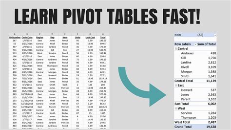
Excel for Mac has been a popular choice among Mac users for its robust features and user-friendly interface. One of the most powerful features of Excel is the pivot table, which enables users to rotate and aggregate data to gain insights and spot trends. Whether you are a student, a business professional, or a data analyst, pivot tables can help you make sense of complex data and make informed decisions.
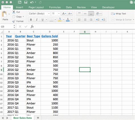
To get started with pivot tables in Excel for Mac, you need to have a dataset that you want to analyze. This dataset can be in the form of a table or a range of cells. Once you have your dataset ready, you can create a pivot table by going to the "Insert" tab in the ribbon and clicking on the "PivotTable" button. This will open the "Create PivotTable" dialog box, where you can select the cell where you want to place the pivot table.
Creating a Pivot Table in Excel for Mac
Creating a pivot table in Excel for Mac is a straightforward process. Here are the steps:
- Select the cell where you want to place the pivot table
- Go to the "Insert" tab in the ribbon
- Click on the "PivotTable" button
- Select the dataset that you want to analyze
- Choose the location where you want to place the pivot table
- Click "OK" to create the pivot table
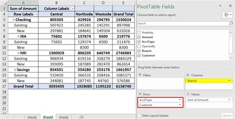
Once you have created the pivot table, you can start customizing it to suit your needs. You can add fields to the pivot table, change the layout, and apply filters to narrow down the data.
Customizing a Pivot Table in Excel for Mac
Customizing a pivot table in Excel for Mac is easy and intuitive. Here are some ways to customize a pivot table:
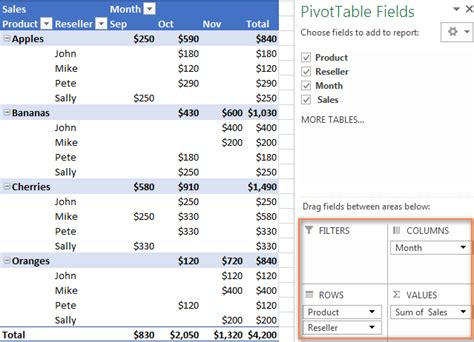
- Add fields to the pivot table by dragging and dropping them from the "PivotTable Fields" pane
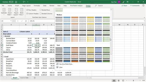
- Change the layout of the pivot table by using the "PivotTable Tools" tab in the ribbon
- Apply filters to the pivot table by using the "Filter" button in the "PivotTable Tools" tab
- Use the "Group" and "Ungroup" buttons to group and ungroup data in the pivot table
Pivot tables can also be used to create charts and graphs. By using the "PivotChart" feature in Excel for Mac, you can create a variety of charts and graphs to visualize your data.
Creating a Pivot Chart in Excel for Mac
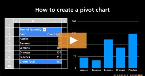
Creating a pivot chart in Excel for Mac is a great way to visualize your data. Here are the steps:
- Select the pivot table that you want to use to create the chart
- Go to the "Insert" tab in the ribbon
- Click on the "PivotChart" button
- Choose the type of chart that you want to create
- Customize the chart as needed
Pivot charts can be used to create a variety of charts and graphs, including column charts, line charts, and pie charts. By using the "PivotChart" feature in Excel for Mac, you can create dynamic and interactive charts that can be used to analyze and present data.
Using Pivot Tables to Analyze Data
Pivot tables can be used to analyze data in a variety of ways. Here are some examples:
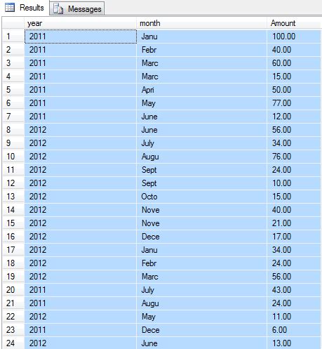
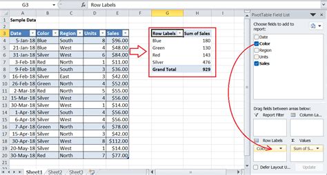
- Summarizing data: Pivot tables can be used to summarize large datasets by using aggregate functions such as SUM, AVERAGE, and COUNT.
- Analyzing trends: Pivot tables can be used to analyze trends in data by using filters and sorting.
- Identifying patterns: Pivot tables can be used to identify patterns in data by using grouping and filtering.
By using pivot tables to analyze data, you can gain insights and spot trends that may not be visible by looking at the raw data. Pivot tables can also be used to create reports and dashboards that can be used to present data to others.
Best Practices for Using Pivot Tables in Excel for Mac
Here are some best practices for using pivot tables in Excel for Mac:
- Use meaningful field names: Use meaningful field names to make it easier to understand the data.
- Use filters: Use filters to narrow down the data and focus on the most important information.
- Use grouping: Use grouping to group related data together.
- Use sorting: Use sorting to sort the data in a logical order.
By following these best practices, you can create effective and efficient pivot tables that can be used to analyze and present data.
Gallery of Pivot Table Examples
Pivot Table Image Gallery


What is a pivot table?
+A pivot table is a tool in Excel that allows users to summarize and analyze large datasets by rotating and aggregating data.
How do I create a pivot table in Excel for Mac?
+To create a pivot table in Excel for Mac, select the cell where you want to place the pivot table, go to the "Insert" tab in the ribbon, click on the "PivotTable" button, select the dataset that you want to analyze, and choose the location where you want to place the pivot table.
What are some common uses of pivot tables?
+Pivot tables can be used to summarize data, analyze trends, identify patterns, and create reports and dashboards.
In conclusion, pivot tables are a powerful tool in Excel for Mac that can be used to summarize and analyze large datasets. By following the steps outlined in this article, you can create and customize pivot tables to suit your needs. Whether you are a student, a business professional, or a data analyst, pivot tables can help you make sense of complex data and make informed decisions. We hope this article has been helpful in guiding you through the process of creating and using pivot tables in Excel for Mac. If you have any further questions or need additional guidance, please don't hesitate to ask.