Index Formula In Cell K9

The INDEX and MATCH functions are two of the most powerful and versatile functions in Excel, allowing users to perform lookups and retrieve data from tables and ranges with great flexibility. When combined, these functions can solve complex data retrieval tasks with ease. Here, we're going to explore how to use the INDEX formula in cell K9, assuming we want to retrieve a specific value based on a criteria or set of criteria.

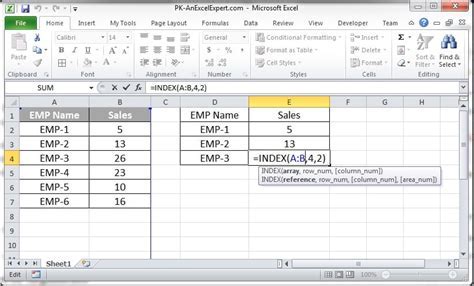
To start, let's understand the basic syntax of the INDEX and MATCH functions. The INDEX function returns a value at a specified position in a range or array. Its syntax is INDEX(range, row_num, col_num), where range is the range of cells, row_num is the relative row position, and col_num is the relative column position. The MATCH function returns the relative position of an item in a range. Its syntax is MATCH(lookup_value, lookup_array, [match_type]), where lookup_value is the value you want to find, lookup_array is the range of cells to search, and match_type specifies whether to look for an exact match or not.

Using INDEX and MATCH for Lookup

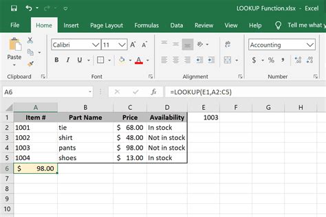
Assuming we have a table with names in column A, ages in column B, and cities in column C, and we want to find the age of a person whose name is mentioned in cell K9, we can use the following formula:

=INDEX(B:B, MATCH(K9, A:A, 0))

This formula looks up the value in cell K9 in column A and returns the corresponding value in column B. Here's how it works:

MATCH(K9, A:A, 0) searches for the value in K9 within column A and returns its relative position.
INDEX(B:B,...) then uses this position to find the corresponding value in column B.

Example with Multiple Criteria

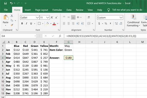
If we need to look up based on multiple criteria (for example, name and city), we can use the INDEX and MATCH functions in combination with the & operator to concatenate the criteria. Let's say we want to find the age of a person whose name is in cell K9 and city is in cell L9. Our formula might look like this:

=INDEX(B:B, MATCH(1, (A:A=K9)*(C:C=L9), 0))

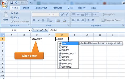
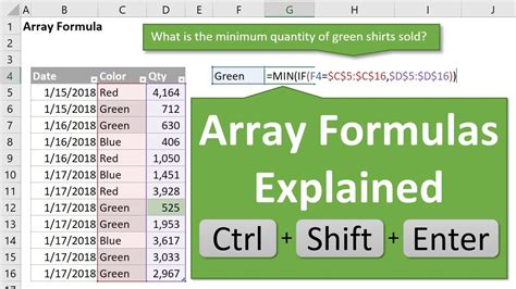
This formula is an array formula, which in older versions of Excel (before Excel 365) requires pressing Ctrl+Shift+Enter instead of just Enter. It works as follows:

(A:A=K9) and (C:C=L9) create arrays of TRUE and FALSE values based on whether the conditions are met.
Multiplying these arrays element-wise with * will result in an array where only the position that meets both conditions will have a TRUE value (since TRUE*TRUE=TRUE and any other combination with FALSE results in FALSE).
MATCH(1,..., 0) then finds the position of this TRUE value, which corresponds to the row where both conditions are met.
Finally, INDEX(B:B,...) returns the value in column B for that row.

Practical Tips

Ensure your data is well-organized and that the lookup values are correctly formatted and not duplicated if you're looking for exact matches.
Use absolute references ($A$1) for the lookup array and range if you plan to copy the formula down or across.
Be mindful of the [match_type] in the MATCH function. A 0 is used for exact matches, 1 for values less than or equal to the lookup value, and -1 for values greater than or equal to the lookup value.

Embedding Images for Illustration

Example of INDEX and MATCH functions in Excel

Gallery of Excel Formulas

Excel Formulas Image Gallery

FAQ Section

What is the purpose of the INDEX function in Excel?

The INDEX function returns a value at a specified position in a range or array.

How does the MATCH function contribute to lookup operations?

The MATCH function returns the relative position of an item in a range, which can then be used by the INDEX function to retrieve a value.

What is the difference between using INDEX/MATCH and VLOOKUP for lookups?

INDEX/MATCH offers more flexibility, especially when looking up values to the left of the return range or performing multiple criteria lookups, whereas VLOOKUP can be simpler but less flexible.

Final Thoughts

Mastering the INDEX and MATCH functions can significantly enhance your Excel skills, allowing you to tackle complex data retrieval tasks with ease. Whether you're working with simple lookups or more intricate multi-criteria searches, understanding how these functions work together can make you more efficient and proficient in Excel. Remember, practice makes perfect, so don't hesitate to experiment with different scenarios and applications of these powerful functions.