Excel Highlight Cell If Greater Than Another Cell

Highlighting cells in Excel based on conditions such as comparing the values of two cells can be incredibly useful for data analysis and visualization. This feature allows you to quickly identify cells that meet certain criteria, making it easier to understand and work with your data. One common requirement is to highlight a cell if its value is greater than another cell. Excel provides a straightforward way to achieve this through Conditional Formatting.

To highlight a cell if its value is greater than another cell, you can follow these steps:

First, it's essential to understand the basics of Conditional Formatting. This feature in Excel enables you to apply specific formatting to a cell or a range of cells based on the cell's value or the value of another cell. You can use it to highlight cells that are greater than, less than, or equal to a specific value, or to compare values between different cells.

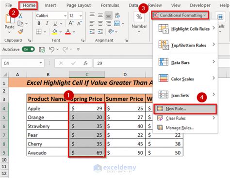
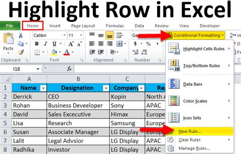
To start, select the cell or range of cells you want to format. This could be a single cell, an entire column, or any range that you're interested in analyzing. Once you've selected your range, go to the Home tab on the Excel ribbon. There, you'll find the Styles group, which includes the Conditional Formatting button.

Click on the Conditional Formatting button to open its menu. This menu offers several options for formatting your cells based on different conditions, including highlighting cells based on their values, using formulas to determine which cells to format, and even creating rules based on the cell's value being above or below average.

For the purpose of highlighting a cell if its value is greater than another cell, you'll want to select "New Rule" from the Conditional Formatting menu. This opens the New Formatting Rule dialog box, where you can define your rule.

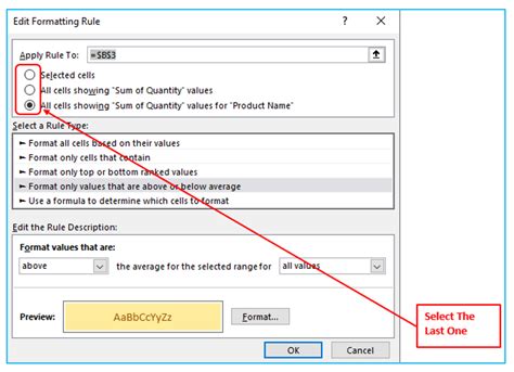
In the New Formatting Rule dialog box, select "Use a formula to determine which cells to format." This option allows you to specify a custom formula that Excel will use to decide whether or not to apply the formatting.

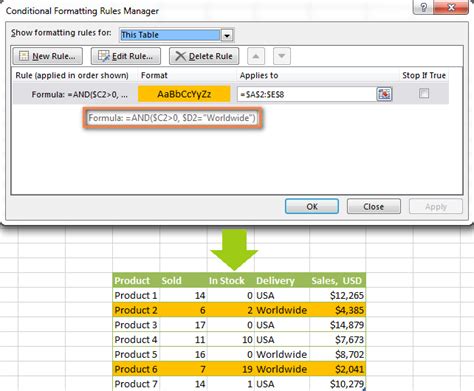
Now, you'll need to enter your formula. If you want to highlight cell A1 if its value is greater than cell B1, your formula would look something like this: =A1>B1. This formula compares the value in cell A1 to the value in cell B1 and returns TRUE if A1 is greater, and FALSE otherwise.

After entering your formula, click on the Format button. This opens the Format Cells dialog box, where you can choose how you want the cells to be formatted when the condition is met. You can select a fill color, change the font color, apply bold or italic formatting, and more.

Once you've selected your formatting options, click OK to apply them and then OK again to close the New Formatting Rule dialog box. Excel will now apply the formatting to any cells in your selected range that meet the condition specified by your formula.

Excel Highlight Cell If Greater Than Another Cell

Benefits of Conditional Formatting

Conditional Formatting offers numerous benefits when working with Excel spreadsheets. It helps in:

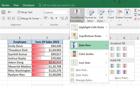
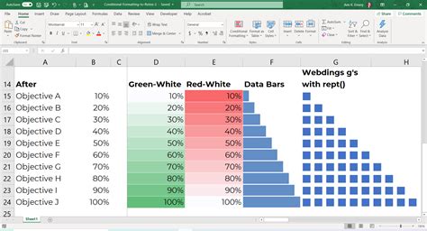
Data Visualization: By applying different formats based on cell values, you can visually distinguish between different types of data, making it easier to analyze and understand.
Error Identification: Formatting rules can be set up to highlight potential errors, such as duplicate values, values outside a specified range, or inconsistencies in formatting.
Data Comparison: As shown, it's useful for comparing values between cells, which can be particularly helpful in financial analysis, statistical analysis, and more.

Step-by-Step Guide to Applying Conditional Formatting

Select the Cell or Range: Click on the cell or select the range of cells you want to apply the formatting rule to.
Open Conditional Formatting: Go to the Home tab on the Excel ribbon, find the Styles group, and click on Conditional Formatting.
Choose New Rule: From the Conditional Formatting dropdown menu, select "New Rule."
Use a Formula: In the New Formatting Rule dialog, choose "Use a formula to determine which cells to format."
Enter the Formula: Type in your formula. For example, to highlight a cell if it's greater than another cell, use =A1>B1.
Format: Click the Format button to choose how you want to format the cells that meet the condition.
Apply: Click OK to apply the rule and see the formatting take effect.

Advanced Conditional Formatting Techniques

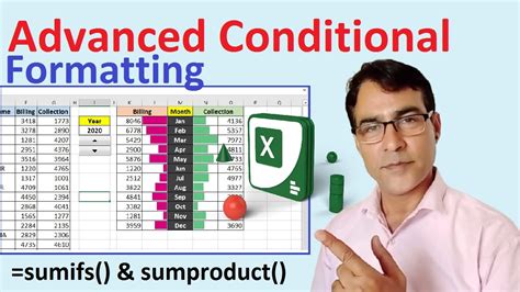
Beyond simple comparisons, Conditional Formatting can handle more complex scenarios, including:

Multiple Conditions: You can apply multiple rules to the same range of cells, allowing for more nuanced formatting based on different conditions.
Relative References: When applying rules, you can use relative references (e.g., A1) that adjust based on the cell being evaluated, making it easier to apply rules across large ranges.
Absolute References: For cases where you want to always compare to a specific cell, you can use absolute references (e.g., $A$1).

Common Uses of Conditional Formatting

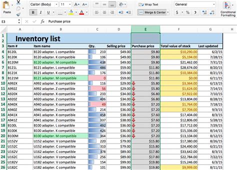
Financial Analysis: Highlighting cells that exceed budget thresholds or identifying negative values in financial reports.
Quality Control: In manufacturing, formatting can be used to highlight defects or quality issues based on inspection data.
Educational Settings: Teachers can use Conditional Formatting to quickly identify students who are above or below certain thresholds in grades or test scores.

Best Practices for Using Conditional Formatting

To get the most out of Conditional Formatting:

Keep it Simple: Avoid overly complex rules that might be hard to understand or maintain.
Use Clear Formulas: Make sure your formulas are easy to read and understand, possibly by using named ranges instead of cell references.
Test Thoroughly: Always test your formatting rules on a small dataset before applying them to larger ranges.

Troubleshooting Conditional Formatting Issues

If your Conditional Formatting rules aren't working as expected:

Check the Formula: Ensure that your formula is correct and references the right cells.
Rule Precedence: Remember that Excel applies rules in the order they appear in the list. If a cell meets the criteria for multiple rules, the first rule applied will take precedence.
Clear Rules: If you're having trouble with conflicting rules, try clearing all rules and starting over.

Conditional Formatting for Data Analysis

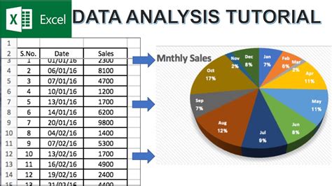
Conditional Formatting is a powerful tool for data analysis, allowing you to visually identify trends, outliers, and patterns within your data. By applying formatting rules based on conditions such as "greater than," "less than," or "between," you can quickly focus on the most critical aspects of your data.

Conclusion and Next Steps

Conditional Formatting in Excel is an indispensable feature for anyone looking to enhance their data analysis and presentation skills. By mastering the art of highlighting cells based on conditions such as being greater than another cell, you can unlock new insights into your data and communicate your findings more effectively. Whether you're working in finance, education, or any other field, the ability to visually distinguish between different types of data can be a game-changer.

Remember, practice makes perfect. The more you work with Conditional Formatting, the more comfortable you'll become with creating complex rules and applying them to real-world scenarios. Don't be afraid to experiment and try out new things – it's all part of the learning process.

Excel Highlight Cell Image Gallery

How do I apply Conditional Formatting in Excel?

To apply Conditional Formatting, select the cell or range of cells, go to the Home tab, click on Conditional Formatting, and choose the type of rule you want to apply.

What are the benefits of using Conditional Formatting?

Conditional Formatting helps in data visualization, error identification, and data comparison, making it easier to analyze and understand data.

Can I apply multiple Conditional Formatting rules to the same range of cells?

Yes, you can apply multiple rules to the same range of cells. Excel will apply these rules in the order they appear in the list.

We hope this comprehensive guide to highlighting cells in Excel if they are greater than another cell has been informative and helpful. Whether you're a seasoned Excel user or just starting out, mastering Conditional Formatting can significantly enhance your productivity and data analysis capabilities. If you have any further questions or would like to explore more advanced Excel features, don't hesitate to reach out or share your experiences in the comments below.