Intro
When working with Excel, being able to look up and retrieve data based on multiple criteria is a crucial skill. This can be particularly challenging when dealing with large datasets where manual searches are impractical. Excel's INDEX and MATCH functions are powerful tools that can be combined to achieve this, allowing users to perform lookups based on multiple conditions. In this article, we will delve into how to use INDEX and MATCH with multiple criteria, exploring the benefits, working mechanisms, and providing practical examples to enhance understanding.
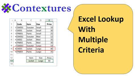
The importance of being able to look up data based on multiple criteria cannot be overstated. In real-world scenarios, data analysis often requires filtering information based on more than one condition. For instance, in a sales database, you might want to find the total sales for a specific product in a particular region. This requires a lookup function that can handle multiple criteria, which is where the combination of INDEX and MATCH comes into play.
Understanding INDEX and MATCH Functions

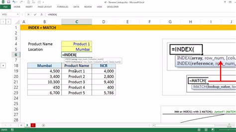
Before diving into using INDEX and MATCH with multiple criteria, it's essential to understand each function individually. The INDEX function returns a value at a specified position in a range or array. The MATCH function returns the position of a value within a range. When used together, they can look up and return a value from an array based on a specified value.
Basic Syntax of INDEX and MATCH
- `INDEX(range, row_num, [col_num])`: Returns a value at the intersection of a row and column. - `MATCH(lookup_value, lookup_array, [match_type])`: Returns the position of a value within a range.Using INDEX and MATCH with Multiple Criteria
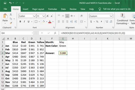
To use INDEX and MATCH with multiple criteria, you'll often employ an array formula, which can handle multiple conditions. The basic approach involves using the MATCH function within an array formula to find the position of the row that meets all the criteria, then using INDEX to return the value from that row.
The formula typically looks like this:
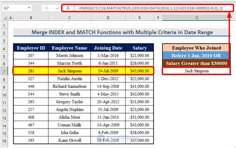
=INDEX(return_range, MATCH(1, (criteria1_range=criteria1) * (criteria2_range=criteria2), 0))
This formula assumes that criteria1_range and criteria2_range are the ranges containing the values to match criteria1 and criteria2, respectively, and return_range is the range from which to return the value.
Practical Example
Suppose you have a database of sales with columns for Region, Product, and Sales Amount, and you want to find the sales amount for a specific product in a particular region.| Region | Product | Sales Amount |
|---|---|---|
| North | A | 100 |
| North | B | 200 |
| South | A | 150 |
| South | B | 250 |
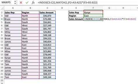
To find the sales amount for Product A in the North region, you could use the following formula:
=INDEX(C2:C5, MATCH(1, (A2:A5="North") * (B2:B5="A"), 0))
Assuming the data is in cells A1:C5, with headers in row 1.
Benefits of Using INDEX and MATCH
Using INDEX and MATCH for lookups offers several benefits, including flexibility, the ability to perform lookups to the left, and avoiding the limitations of the VLOOKUP function. Additionally, these functions can handle multiple criteria with ease, making them indispensable for complex data analysis tasks.
Common Errors and Troubleshooting
When working with `INDEX` and `MATCH`, especially with multiple criteria, common issues include incorrect range references, mismatched data types, and forgetting to enter the formula as an array formula (by pressing `Ctrl+Shift+Enter` instead of just `Enter`).Advanced Applications and Alternatives
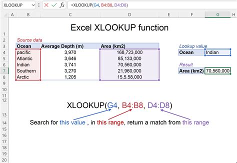
For more complex scenarios, or when working with very large datasets, alternatives like XLOOKUP (available in newer versions of Excel) or using pivot tables might offer more efficient solutions. XLOOKUP simplifies the lookup process and can handle multiple criteria more intuitively than INDEX and MATCH.
Gallery of Excel Lookup Functions
Excel Lookup Functions Image Gallery


Frequently Asked Questions
What is the main difference between VLOOKUP and INDEX/MATCH?
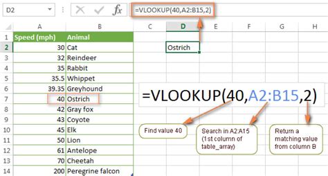
+The main difference is that VLOOKUP looks up a value in the first column of a table and returns a value in the same row from another column, whereas INDEX/MATCH offers more flexibility, including looking up values to the left and handling multiple criteria more gracefully.
How do I handle multiple criteria with INDEX and MATCH?
+To handle multiple criteria, you use an array formula that multiplies the conditions together. For example, (criteria1_range=criteria1) * (criteria2_range=criteria2) within the MATCH function.
What are some common errors when using INDEX and MATCH?
+Common errors include incorrect range references, forgetting to enter the formula as an array formula, and mismatched data types between the criteria and the range being searched.
In conclusion, mastering the use of INDEX and MATCH with multiple criteria is a valuable skill for anyone working with Excel, offering a powerful and flexible way to perform lookups and data analysis. Whether you're dealing with simple datasets or complex databases, understanding how to leverage these functions can significantly enhance your productivity and capabilities in Excel. We invite you to share your experiences or ask questions about using INDEX and MATCH in the comments below, and don't forget to share this article with others who might benefit from learning about these essential Excel functions.