Intro
When working with Excel pivot tables, it's common to encounter situations where certain items or fields appear to be missing from the table. This can happen for a variety of reasons, such as the data not being populated for those specific items or the pivot table settings filtering them out. One of the challenges users face is how to show items with no data in an Excel pivot table, ensuring that all relevant information, including empty or null values, is visible and accounted for. This can be particularly useful for analysis, reporting, and ensuring data integrity.
To address this issue, Excel provides several approaches that allow users to display items with no data in their pivot tables. Understanding and applying these methods can significantly enhance the usability and analytical capability of pivot tables.
Understanding Pivot Tables
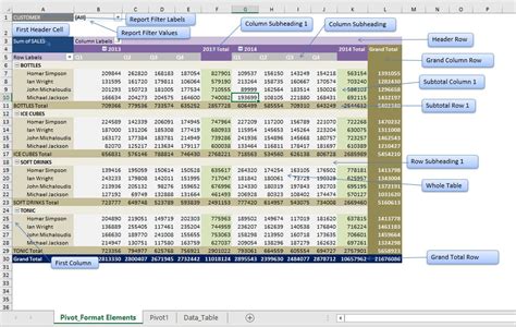
Before diving into the solutions, it's essential to have a basic understanding of pivot tables. Pivot tables are a powerful tool in Excel that allows users to summarize, analyze, and visualize large datasets. They enable users to rotate and aggregate data, making it easier to understand and draw insights from the data.
Displaying Items with No Data
The primary method to display items with no data involves adjusting the pivot table settings. Here's how you can do it:
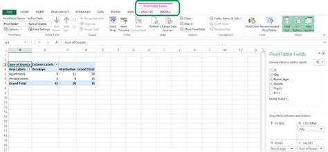
- Select the Pivot Table: Click anywhere on the pivot table to select it. This action will activate the PivotTable Tools tabs in the ribbon.
- Go to PivotTable Options: In the PivotTable Tools, navigate to the "Analyze" tab (or "Options" tab in older Excel versions), and click on the "Options" button in the PivotTable group. This will open the PivotTable Options dialog box.
- Display Items with No Data: In the PivotTable Options dialog box, go to the "Display" tab. Check the box next to "Show items with no data on rows" and/or "Show items with no data on columns," depending on whether you want to display items with no data in your rows or columns.
- Apply Changes: Click "OK" to apply these changes. Your pivot table should now display items that have no data associated with them.
Additional Tips for Managing Pivot Table Data
- Filtering: Sometimes, the data you're looking for might be hidden due to filters applied to the pivot table or its fields. Make sure to check the filters and clear any that might be excluding the data you need.
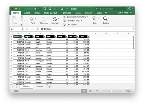
- Data Source: Ensure that your data source includes all the items you expect to see in the pivot table. If items are missing from the source data, they won't appear in the pivot table, even with the "Show items with no data" option enabled.
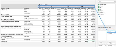
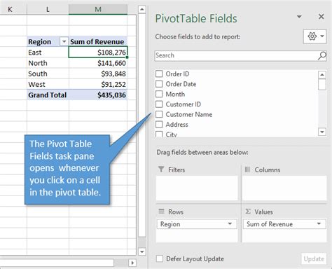
- Pivot Table Fields: The fields you drag into the "Rows," "Columns," "Values," and "Filters" areas of the pivot table can significantly affect what data is displayed. Experiment with different field placements to achieve the desired view.
Using Pivot Table Settings for Empty Cells
When dealing with empty cells in a pivot table, you might also want to consider how these are displayed. By default, Excel shows empty cells as blank, but you can change this setting:
- Go to Options: Follow the same steps as before to open the PivotTable Options dialog box.
- For empty cells: In the "Layout & Format" tab, look for the "For empty cells show:" option. You can enter a custom value here, such as "0" or "N/A," to replace the blank cells.
Practical Applications and Examples
Displaying items with no data can be crucial in various scenarios, such as:
- Inventory Management: When tracking inventory levels, showing items with no data (i.e., out-of-stock items) can help in identifying which products need restocking.
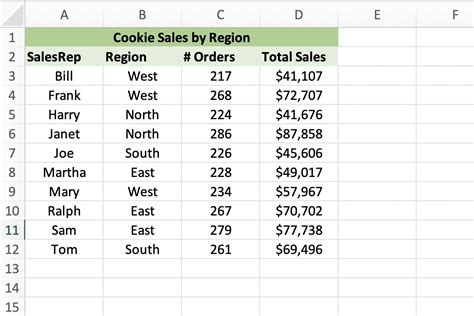
- Sales Analysis: In sales reports, displaying regions or products with no sales data can highlight areas that require more marketing effort or indicate discontinued products.
Gallery of Pivot Table Customization
Gallery of Excel Pivot Tables
Pivot Table Image Gallery


FAQs
How do I show all items in a pivot table, even if they have no data?
+To show all items in a pivot table, including those with no data, you need to adjust the pivot table options. Select the pivot table, go to the "Analyze" tab, click on "Options," then in the PivotTable Options dialog box, check the boxes for "Show items with no data on rows" and/or "Show items with no data on columns" in the "Display" tab.
Why are some items missing from my pivot table?
+Items might be missing from your pivot table due to several reasons: they might be filtered out, the data source might not include them, or the pivot table settings might be hiding them. Check your filters, data source, and pivot table settings to ensure all necessary items are included and visible.
How can I change what is displayed in empty cells of a pivot table?
+To change what is displayed in empty cells, go to the PivotTable Options dialog box, navigate to the "Layout & Format" tab, and enter a value in the "For empty cells show:" field. This allows you to replace blank cells with a custom value, such as "0" or "N/A."
In conclusion, displaying items with no data in Excel pivot tables is a valuable skill for anyone working with data analysis and reporting. By understanding how to adjust pivot table settings and customize the display of empty cells, users can create more comprehensive and informative reports. Whether you're working in inventory management, sales analysis, or any other field that relies on data insights, mastering these techniques can significantly enhance your ability to extract meaningful information from your data. If you have any questions or need further clarification on how to work with pivot tables, don't hesitate to reach out. Share your experiences or tips on working with pivot tables in the comments below, and consider sharing this article with others who might benefit from learning more about Excel's powerful pivot table features.