Google Sheets Conditional Formatting Whole Row Based On One Cell

Conditional formatting in Google Sheets is a powerful tool that allows users to highlight cells based on specific conditions, making it easier to visualize and analyze data. One common requirement is to apply conditional formatting to an entire row based on the value of a single cell within that row. This can be particularly useful for drawing attention to specific rows that meet certain criteria, such as deadlines, priorities, or specific statuses.

To apply conditional formatting to a whole row based on one cell in Google Sheets, follow these steps:

First, it's essential to understand the basic principles of conditional formatting. Conditional formatting allows you to change the appearance of cells based on their values, formulas, or formatting. You can apply various formatting options, including background color, font color, and more, to cells that meet specific conditions.

Steps to Conditionally Format a Whole Row

1. Select the Range: Start by selecting the entire range of cells that you want to format. If you want to format the entire row based on a condition in one cell, select the whole row. For example, if your data starts from row 1 and you want to apply the formatting to rows 1 through 100, select cells A1:Z100 (assuming your data spans from column A to Z).

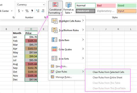
2. Open Conditional Formatting: With your range selected, go to the "Format" tab in the menu, then click on "Conditional formatting."

3. Apply Custom Formula: In the conditional formatting panel, you will see several options for applying formatting based on cell values, formulas, and more. For applying formatting to a whole row based on one cell, you will typically use a custom formula.

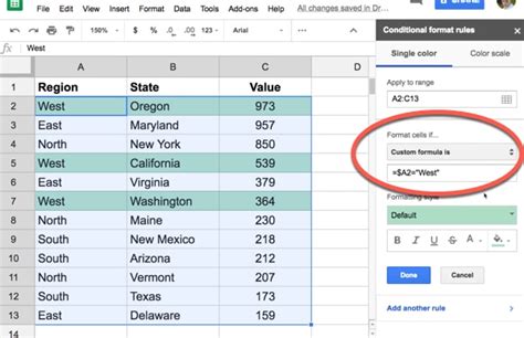
4. Custom Formula: In the format cells if dropdown, select "Custom formula is." Then, in the formula bar, you can enter a formula that refers to the cell you want to base your formatting on. For example, if you want to highlight the entire row if the value in column A is "Yes," you could use the formula =$A1="Yes".

5. Apply to Range: Make sure the range you selected initially is correctly reflected in the "Apply to range" field. If you're applying this to rows 1 through 100, it should show A1:Z100.

6. Format: Choose the formatting you want to apply. You can change the background color, text color, and more.

7. Done: Click "Done" to apply your conditional formatting rule.

Example Use Cases

• Highlighting Overdue Tasks: If you have a project management spreadsheet where one column indicates the status of tasks (e.g., "Overdue"), you can use conditional formatting to highlight the entire row for tasks that are overdue, making it easier to identify which tasks need immediate attention.

• Prioritizing Tasks: Similarly, if you have a column for priority levels (e.g., "High," "Medium," "Low"), you can apply conditional formatting to highlight rows with high-priority tasks.

• Identifying Completed Tasks: For a to-do list or task management sheet, you might want to apply a specific formatting to rows where the task is marked as "Completed," helping you visually distinguish between completed and pending tasks.

Tips and Variations

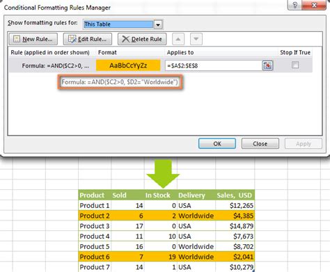
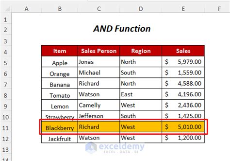
• Using Multiple Conditions: You can also apply multiple conditions by using the AND or OR functions within your custom formula. For example, to highlight rows where the value in column A is "Yes" and the value in column B is greater than 10, you could use =AND($A1="Yes", $B1>10).

• Applying to Entire Columns: If you want to apply the formatting based on the condition in one cell but to the entire column instead of the row, you can adjust the range and formula accordingly.

• Dynamic Range: For dynamic ranges that may change (e.g., as you add more data), consider using named ranges or referencing the entire column/row in your formula.

By leveraging conditional formatting based on specific cell values, you can significantly enhance the readability and usability of your Google Sheets, making it easier to analyze, prioritize, and act upon the data within them.

Advanced Conditional Formatting Techniques

For more complex scenarios, you might need to combine multiple conditions, use regular expressions, or even apply formatting based on the formatting of other cells. Google Sheets' conditional formatting is quite powerful and can handle these advanced scenarios with the right formulas and techniques.

Common Conditional Formatting Formulas

Here are a few examples of common conditional formatting formulas you might find useful:

• Greater Than: =$A1>10
• Less Than: =$A1<10
• Equal To: =$A1="Yes"
• Not Equal To: =$A1<>"No"
• Between: =AND($A1>10, $A1<20)
• Outside Range: =OR($A1<10, $A1>20)

These formulas can be adapted and combined to fit a wide range of conditions and scenarios.

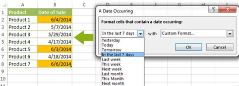
Conditional Formatting for Dates

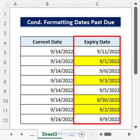
Conditional formatting can also be applied based on dates. For example, you might want to highlight cells that contain today's date, yesterday's date, or dates within a specific range.

• Today's Date: =TODAY()
• Yesterday's Date: =TODAY()-1
• Within the Next 7 Days: =AND(A1>=TODAY(), A1<=TODAY()+7)

These date-based conditions can be particularly useful in calendars, schedules, and project timelines.

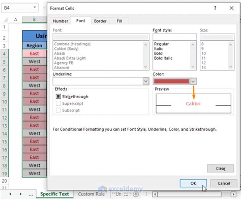
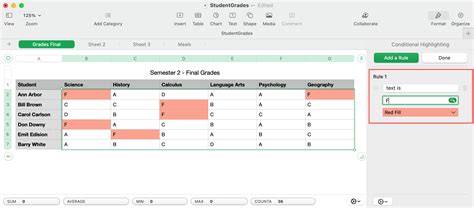
Conditional Formatting for Text

For text-based conditions, you can use formulas that check for specific words, phrases, or patterns within the text.

• Contains a Specific Word: =REGEXMATCH(A1, "word")
• Starts With: =REGEXMATCH(A1, "^word")
• Ends With: =REGEXMATCH(A1, "word

  Conditional formatting in Google Sheets is a powerful tool that allows users to highlight cells based on specific conditions, making it easier to visualize and analyze data. One common requirement is to apply conditional formatting to an entire row based on the value of a single cell within that row. This can be particularly useful for drawing attention to specific rows that meet certain criteria, such as deadlines, priorities, or specific statuses.

  To apply conditional formatting to a whole row based on one cell in Google Sheets, follow these steps:

  First, it's essential to understand the basic principles of conditional formatting. Conditional formatting allows you to change the appearance of cells based on their values, formulas, or formatting. You can apply various formatting options, including background color, font color, and more, to cells that meet specific conditions.

  Steps to Conditionally Format a Whole Row

  1. Select the Range: Start by selecting the entire range of cells that you want to format. If you want to format the entire row based on a condition in one cell, select the whole row. For example, if your data starts from row 1 and you want to apply the formatting to rows 1 through 100, select cells A1:Z100 (assuming your data spans from column A to Z).

  2. Open Conditional Formatting: With your range selected, go to the "Format" tab in the menu, then click on "Conditional formatting."

  3. Apply Custom Formula: In the conditional formatting panel, you will see several options for applying formatting based on cell values, formulas, and more. For applying formatting to a whole row based on one cell, you will typically use a custom formula.

  4. Custom Formula: In the format cells if dropdown, select "Custom formula is." Then, in the formula bar, you can enter a formula that refers to the cell you want to base your formatting on. For example, if you want to highlight the entire row if the value in column A is "Yes," you could use the formula =$A1="Yes".

  5. Apply to Range: Make sure the range you selected initially is correctly reflected in the "Apply to range" field. If you're applying this to rows 1 through 100, it should show A1:Z100.

  6. Format: Choose the formatting you want to apply. You can change the background color, text color, and more.

  7. Done: Click "Done" to apply your conditional formatting rule.

  Example Use Cases

  • Highlighting Overdue Tasks: If you have a project management spreadsheet where one column indicates the status of tasks (e.g., "Overdue"), you can use conditional formatting to highlight the entire row for tasks that are overdue, making it easier to identify which tasks need immediate attention.

  • Prioritizing Tasks: Similarly, if you have a column for priority levels (e.g., "High," "Medium," "Low"), you can apply conditional formatting to highlight rows with high-priority tasks.

  • Identifying Completed Tasks: For a to-do list or task management sheet, you might want to apply a specific formatting to rows where the task is marked as "Completed," helping you visually distinguish between completed and pending tasks.

  Tips and Variations

  • Using Multiple Conditions: You can also apply multiple conditions by using the AND or OR functions within your custom formula. For example, to highlight rows where the value in column A is "Yes" and the value in column B is greater than 10, you could use =AND($A1="Yes", $B1>10).

  • Applying to Entire Columns: If you want to apply the formatting based on the condition in one cell but to the entire column instead of the row, you can adjust the range and formula accordingly.

  • Dynamic Range: For dynamic ranges that may change (e.g., as you add more data), consider using named ranges or referencing the entire column/row in your formula.

  By leveraging conditional formatting based on specific cell values, you can significantly enhance the readability and usability of your Google Sheets, making it easier to analyze, prioritize, and act upon the data within them.

  

  Advanced Conditional Formatting Techniques

  For more complex scenarios, you might need to combine multiple conditions, use regular expressions, or even apply formatting based on the formatting of other cells. Google Sheets' conditional formatting is quite powerful and can handle these advanced scenarios with the right formulas and techniques.

  Common Conditional Formatting Formulas

  

  Here are a few examples of common conditional formatting formulas you might find useful:

  • Greater Than: =$A1>10
  • Less Than: =$A1<10
  • Equal To: =$A1="Yes"
  • Not Equal To: =$A1<>"No"
  • Between: =AND($A1>10, $A1<20)
  • Outside Range: =OR($A1<10, $A1>20)

  These formulas can be adapted and combined to fit a wide range of conditions and scenarios.

  Conditional Formatting for Dates

  

  Conditional formatting can also be applied based on dates. For example, you might want to highlight cells that contain today's date, yesterday's date, or dates within a specific range.

  • Today's Date: =TODAY()
  • Yesterday's Date: =TODAY()-1
  • Within the Next 7 Days: =AND(A1>=TODAY(), A1<=TODAY()+7)

  These date-based conditions can be particularly useful in calendars, schedules, and project timelines.

  Conditional Formatting for Text

  

  For text-based conditions, you can use formulas that check for specific words, phrases, or patterns within the text.

  • Contains a Specific Word: =REGEXMATCH(A1, "word")
  • Starts With: =REGEXMATCH(A1, "^word")
  • Ends With: =REGEXMATCH(A1, "word${content}quot;)

  These text-based conditions are useful for categorizing, filtering, or highlighting specific types of data based on their textual content.

  Gallery of Conditional Formatting Examples

  Conditional Formatting Image Gallery

  

  

  

  

  

  

  

  

  

  

  Frequently Asked Questions

  How do I apply conditional formatting to an entire row based on one cell?

  +

  Select the range you want to format, go to the "Format" tab, click on "Conditional formatting," and then use a custom formula that references the cell you want to base your formatting on.

  Can I apply multiple conditions to the same range?

  +

  Yes, you can apply multiple conditions by using the "AND" or "OR" functions within your custom formula.

  How do I format cells based on dates?

  +

  You can use formulas that reference the "TODAY()" function or specific date ranges to format cells based on dates.

  In conclusion, conditional formatting is a versatile and powerful feature in Google Sheets that can significantly enhance your data analysis and presentation capabilities. By mastering the techniques for applying conditional formatting to whole rows based on specific cell values, you can unlock new ways to visualize, categorize, and interact with your data. Whether you're working with dates, numbers, or text, conditional formatting provides a flexible and dynamic way to make your spreadsheets more informative and user-friendly. So, don't hesitate to explore and apply these techniques to your Google Sheets projects, and discover how conditional formatting can revolutionize your workflow and productivity.

  quot;)

These text-based conditions are useful for categorizing, filtering, or highlighting specific types of data based on their textual content.

Gallery of Conditional Formatting Examples

Conditional Formatting Image Gallery

Frequently Asked Questions

How do I apply conditional formatting to an entire row based on one cell?

+

Select the range you want to format, go to the "Format" tab, click on "Conditional formatting," and then use a custom formula that references the cell you want to base your formatting on.

Can I apply multiple conditions to the same range?

+

Yes, you can apply multiple conditions by using the "AND" or "OR" functions within your custom formula.

How do I format cells based on dates?

+

You can use formulas that reference the "TODAY()" function or specific date ranges to format cells based on dates.

In conclusion, conditional formatting is a versatile and powerful feature in Google Sheets that can significantly enhance your data analysis and presentation capabilities. By mastering the techniques for applying conditional formatting to whole rows based on specific cell values, you can unlock new ways to visualize, categorize, and interact with your data. Whether you're working with dates, numbers, or text, conditional formatting provides a flexible and dynamic way to make your spreadsheets more informative and user-friendly. So, don't hesitate to explore and apply these techniques to your Google Sheets projects, and discover how conditional formatting can revolutionize your workflow and productivity.