Intro
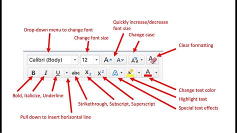
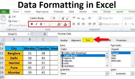
Learn to format fonts in Excel using formulas, including font size, color, and style, with conditional formatting and formula-based font changes.
Formatting fonts in Excel can greatly enhance the readability and visual appeal of your spreadsheets. While Excel provides various formatting options through its user interface, using formulas to format fonts can offer more flexibility and automation. In this article, we will delve into the world of conditional formatting and explore how to use formulas to change font colors, sizes, and styles in Excel.
Excel is a powerful tool used for data analysis, budgeting, and more. Its ability to format cells based on specific conditions makes it an indispensable tool for professionals and individuals alike. One of the key features of Excel is its ability to use formulas for conditional formatting. This feature allows users to change the appearance of cells based on the values in those cells or in other cells.
Conditional formatting is a feature in Excel that allows you to apply formatting to a cell or a range of cells based on certain conditions or criteria. You can use formulas to specify these conditions, making it possible to dynamically change the formatting of cells based on the data in your spreadsheet. For instance, you can use a formula to highlight cells that contain a specific value, or to change the font color of cells that meet a certain condition.
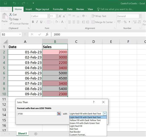
To get started with using formulas for font formatting in Excel, you need to understand how conditional formatting works. Conditional formatting is applied through the "Home" tab in the Excel ribbon, under the "Styles" group. Here, you can find the "Conditional Formatting" button, which opens a dropdown menu with various options, including "New Rule." This is where you can input your custom formula to format fonts.
Using Formulas for Conditional Formatting
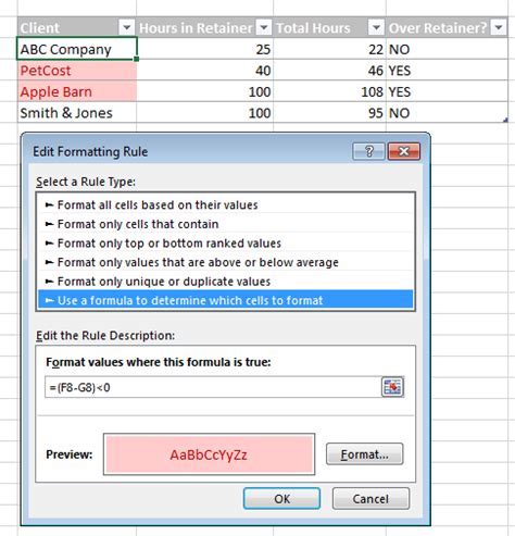
When you choose to create a new rule, you have the option to "Use a formula to determine which cells to format." This option allows you to input a formula that, if true, will apply the specified formatting to the cell. For example, if you want to change the font color of all cells in column A that contain the word "example," you can use a formula like =ISNUMBER(SEARCH("example",A1)). This formula checks if the cell A1 contains the word "example" and, if so, applies the formatting.
Steps to Apply Conditional Formatting with Formulas
To apply conditional formatting based on a formula, follow these steps: 1. Select the range of cells you want to format. 2. Go to the "Home" tab in the Excel ribbon. 3. Click on "Conditional Formatting" in the "Styles" group. 4. Choose "New Rule." 5. Select "Use a formula to determine which cells to format." 6. Enter your formula in the formula bar. 7. Click on the "Format" button to choose the formatting you want to apply. 8. Click "OK" to apply the rule.Common Formulas for Font Formatting
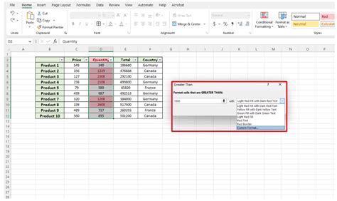
There are several common scenarios where you might want to use formulas to format fonts in Excel. For instance, you might want to highlight cells that are greater than a certain value, or change the font color of cells that contain specific text. Here are a few examples of formulas you can use:
=A1>10to format cells in column A that are greater than 10.=ISNUMBER(SEARCH("text",A1))to format cells in column A that contain the word "text."=TODAY()-A1>30to format cells in column A that are more than 30 days old.
Advanced Formulas for Conditional Formatting
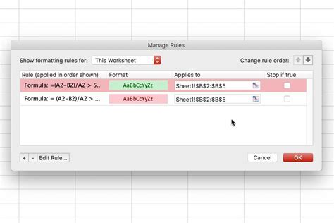
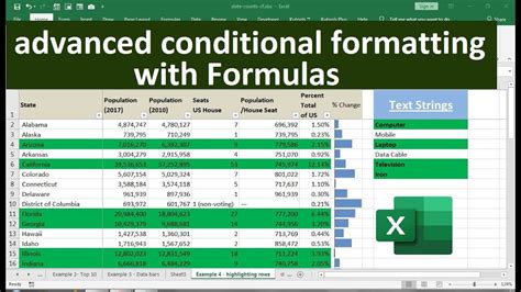
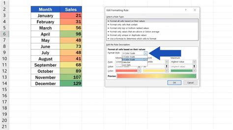
For more complex conditions, you can use advanced formulas that combine multiple criteria. For example, you can use the `AND` or `OR` functions to apply formatting based on multiple conditions. The syntax for these functions is as follows: - `AND(condition1, condition2,...)` returns true if all conditions are true. - `OR(condition1, condition2,...)` returns true if any condition is true.Using these functions, you can create complex rules for formatting your cells. For instance, =AND(A1>10, B1="example") will format cells in column A that are greater than 10 and have the word "example" in the corresponding cell in column B.
Best Practices for Using Formulas in Conditional Formatting
When using formulas for conditional formatting, there are a few best practices to keep in mind:
- Keep your formulas simple and easy to understand. Complex formulas can be difficult to maintain and debug.
- Use absolute references (
$A$1) when you want to refer to a specific cell, and relative references (A1) when you want the formula to adjust based on the cell being formatted. - Test your formulas thoroughly to ensure they are working as expected.
Troubleshooting Common Issues
Sometimes, your conditional formatting rules may not work as expected. Here are a few common issues and how to troubleshoot them: - If your formatting is not being applied, check that your formula is correct and that the formatting options are set correctly. - If your formatting is being applied to the wrong cells, check that your formula is referencing the correct cells and that you have selected the correct range of cells to format.Gallery of Conditional Formatting Examples
Conditional Formatting Image Gallery


Frequently Asked Questions
What is conditional formatting in Excel?
+Conditional formatting is a feature in Excel that allows you to apply formatting to a cell or a range of cells based on certain conditions or criteria.
How do I use formulas for conditional formatting?
+To use formulas for conditional formatting, select the range of cells you want to format, go to the "Home" tab, click on "Conditional Formatting," choose "New Rule," and then select "Use a formula to determine which cells to format."
What are some common formulas used for conditional formatting?
+Common formulas include `=A1>10` to format cells greater than 10, `=ISNUMBER(SEARCH("text",A1))` to format cells containing specific text, and `=TODAY()-A1>30` to format cells that are more than 30 days old.
How do I troubleshoot issues with conditional formatting?
+To troubleshoot issues, check that your formula is correct, the formatting options are set correctly, and the correct range of cells is selected. Also, ensure that your formula references the correct cells and adjust as necessary.
What are some best practices for using formulas in conditional formatting?
+Best practices include keeping formulas simple, using absolute references when necessary, and testing formulas thoroughly to ensure they work as expected.
In conclusion, using formulas for font formatting in Excel can greatly enhance the functionality and readability of your spreadsheets. By understanding how to apply conditional formatting based on formulas, you can automate the process of highlighting important information, making your data more intuitive and easier to analyze. Whether you're a professional data analyst or just starting to explore the capabilities of Excel, mastering the use of formulas for conditional formatting can take your spreadsheet skills to the next level. So, take the time to practice and experiment with different formulas and formatting options to see how you can leverage this powerful feature to improve your work with Excel. If you have any questions or need further clarification on any of the topics covered, don't hesitate to reach out. Share your experiences and tips for using formulas in conditional formatting in the comments below, and help build a community of Excel users who can learn from and support each other.