How To Create A Pivot Table In Excel By Month

Pivot tables are a powerful tool in Excel that allows users to summarize and analyze large datasets with ease. One common requirement is to create a pivot table that shows data by month. This can be particularly useful for tracking sales, expenses, or other metrics over time. In this article, we will walk through the steps to create a pivot table in Excel by month.

Creating a pivot table by month can help you identify trends and patterns in your data that may not be immediately apparent. For example, you may notice that sales are higher in certain months or that expenses tend to peak during specific periods. By analyzing your data in this way, you can make more informed decisions about your business or organization.

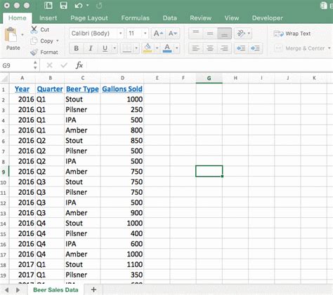
To get started, you will need a dataset that includes a date field. This can be a column of dates in the format mm/dd/yyyy or any other format that Excel recognizes as a date. You will also need to have Excel 2013 or later installed on your computer, as earlier versions of Excel do not support the pivot table features we will be using.

Preparing Your Data

Before you can create a pivot table, you need to make sure your data is properly formatted. This includes ensuring that your date field is in a format that Excel recognizes as a date. You can check this by selecting the entire column and looking at the format in the Number group of the Home tab. If the format is not already set to a date format, you can change it by selecting the format you want from the dropdown list.

You should also make sure that your data is organized in a table format, with each row representing a single record and each column representing a field. This will make it easier to create the pivot table and ensure that your data is summarized correctly.

Creating The Pivot Table

To create the pivot table, select the entire dataset and go to the Insert tab. Click on the PivotTable button and select a cell where you want the pivot table to be placed. You can choose to place the pivot table in a new worksheet or in an existing one.

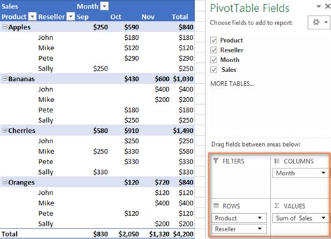
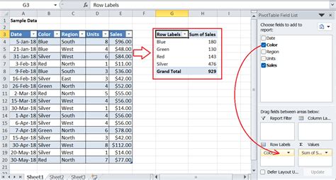
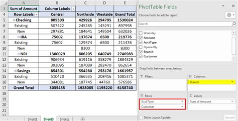
Once you have selected the location for the pivot table, click OK to create it. The pivot table will be empty at first, but you can start adding fields to it by dragging them from the PivotTable Fields pane to the different areas of the pivot table.

Adding Fields To The Pivot Table

To create a pivot table by month, you need to add the date field to the Row Labels area of the pivot table. You can do this by dragging the date field from the PivotTable Fields pane to the Row Labels area.

You will also need to add a field to the Values area of the pivot table. This can be a field that contains numerical data, such as sales or expenses. You can add multiple fields to the Values area if you want to summarize different metrics.

Grouping Dates By Month

To group the dates by month, right-click on the date field in the Row Labels area and select Group. In the Grouping dialog box, select Months and click OK. This will group the dates by month, and the pivot table will be updated to show the summarized data for each month.

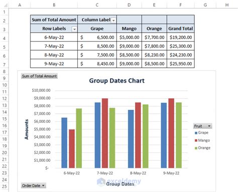
You can also use the Date Grouping feature to group dates by quarter or year. This can be useful if you want to analyze your data over a longer period of time.

Customizing The Pivot Table

Once you have created the pivot table, you can customize it to suit your needs. You can add or remove fields, change the layout, and apply filters to the data.

You can also use the pivot table to create charts and other visualizations. This can help you to better understand your data and identify trends and patterns.

Common Pitfalls To Avoid

When creating a pivot table, there are several common pitfalls to avoid. One of the most common mistakes is not properly formatting the data before creating the pivot table. This can lead to errors and inconsistencies in the pivot table.

Another common mistake is not using the correct fields in the pivot table. This can result in incorrect summaries and analyses.

You should also avoid using too many fields in the pivot table, as this can make it difficult to understand and analyze the data.

Tips And Tricks

Here are some tips and tricks to help you get the most out of your pivot table:

• Use the pivot table to create charts and other visualizations.
• Apply filters to the data to focus on specific subsets of the data.
• Use the Date Grouping feature to group dates by month, quarter, or year.
• Use multiple fields in the Values area to summarize different metrics.

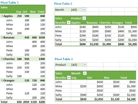
Gallery of Pivot Table Examples

Pivot Table Image Gallery

Frequently Asked Questions

What is a pivot table?

+

A pivot table is a powerful tool in Excel that allows users to summarize and analyze large datasets with ease.

How do I create a pivot table in Excel?

+

To create a pivot table, select the entire dataset and go to the Insert tab. Click on the PivotTable button and select a cell where you want the pivot table to be placed.

How do I group dates by month in a pivot table?

+

To group dates by month, right-click on the date field in the Row Labels area and select Group. In the Grouping dialog box, select Months and click OK.

In conclusion, creating a pivot table in Excel by month can be a powerful way to analyze and summarize your data. By following the steps outlined in this article, you can create a pivot table that shows your data by month and gain valuable insights into your business or organization. We encourage you to try out the techniques described in this article and to experiment with different ways of using pivot tables to analyze your data. If you have any questions or need further assistance, please don't hesitate to comment below or share this article with others who may find it helpful.