How To Create Min Max Average Graph In Excel

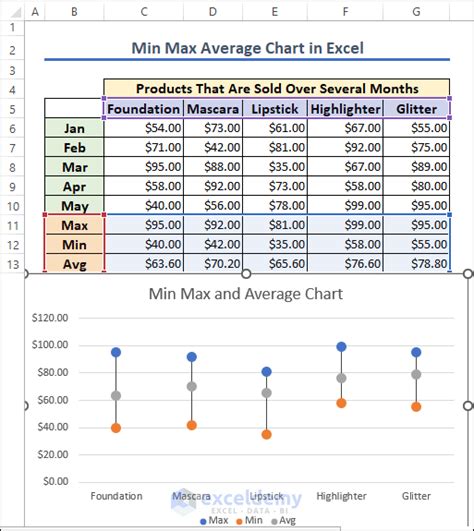
Creating a min max average graph in Excel is a useful way to visualize and compare data, helping to identify trends, patterns, and outliers. This type of graph is particularly useful in statistical analysis, quality control, and financial analysis. To create a min max average graph in Excel, follow these steps, which will guide you through the process of preparing your data, setting up the chart, and customizing it to meet your needs.

Understanding the importance of data visualization, Excel provides a variety of tools and charts to help present data in a meaningful way. The min max average graph, also known as a min-max-average chart or a range chart, displays the minimum, maximum, and average values of a dataset. This can be particularly useful for showing how data points vary over time or across different categories.

Before diving into the steps to create the graph, it's essential to understand the benefits of using such a graph. The min max average graph allows for the quick identification of data points that are significantly higher or lower than the average, which can indicate anomalies or trends worth further investigation. Additionally, by comparing the range (the difference between the maximum and minimum values) across different datasets or time periods, you can assess variability and stability.

To start creating your min max average graph, ensure your data is well-organized. Typically, your data should be arranged in a table with categories in one column and corresponding values in another. If your data is not already in a table format, consider converting it into one for easier manipulation and analysis.

Preparing Your Data

Preparing Data for Min Max Average Graph

Preparing your data is the first step in creating a min max average graph. Ensure that your data is clean, consistent, and well-organized. This might involve removing any unnecessary columns or rows, handling missing data, and ensuring that your data categories are clearly defined. Excel's data manipulation tools, such as filtering, sorting, and pivot tables, can be very helpful in this stage.

Calculating Min, Max, and Average

Once your data is prepared, you'll need to calculate the minimum, maximum, and average values for each category. Excel provides formulas for these calculations: MIN(range), MAX(range), and AVERAGE(range), where "range" refers to the set of cells containing your data. You can also use the AutoSum feature to quickly insert these formulas.

Using Formulas for Calculations

MIN Formula: =MIN(A1:A10) calculates the smallest number in the range A1 through A10.
MAX Formula: =MAX(A1:A10) calculates the largest number in the range A1 through A10.
AVERAGE Formula: =AVERAGE(A1:A10) calculates the average of the numbers in the range A1 through A10.

These formulas can be applied to each category of your data to get the minimum, maximum, and average values.

Creating the Chart

After calculating the min, max, and average values, you're ready to create the chart. Here’s how:

Select Your Data: Choose the cells that contain your category labels and the calculated min, max, and average values.
Insert Chart: Go to the "Insert" tab on the Excel ribbon, click on "Chart," and select the type of chart that best suits your data. For a min max average graph, a line chart or a combination chart might be appropriate.
Customize Your Chart: Use the "Chart Design" and "Chart Format" tabs to customize the appearance of your chart. You can change colors, add titles, and adjust the axis labels to make your chart more informative and visually appealing.

Customizing the Chart

Customization is key to making your chart effective. Consider the following steps:

Add a Title: Clearly describe what your chart represents.
Label Axes: Ensure that your x and y axes are labeled appropriately.
Use Legends: If you have multiple lines or series in your chart, use a legend to distinguish between them.
Adjust Scales: Make sure the scale of your y-axis appropriately reflects the range of your data.

Interpreting Your Chart

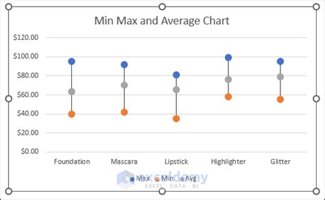
Once your chart is created and customized, it's time to interpret the results. Look for patterns, trends, and outliers. The min max average graph can help you understand the variability of your data and how it changes over time or across different categories.

Identifying Trends and Outliers

Trends: Look for consistent patterns in how the minimum, maximum, and average values change.
Outliers: Identify any data points that are significantly higher or lower than the average, indicating potential anomalies.

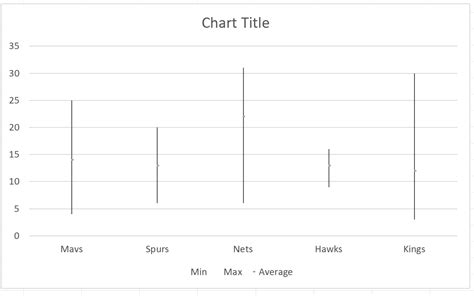
Gallery of Min Max Average Graphs

Min Max Average Graph Examples

Frequently Asked Questions

What is a Min Max Average Graph?

A min max average graph is a type of chart that displays the minimum, maximum, and average values of a dataset, helping to visualize variability and trends.

How Do I Create a Min Max Average Graph in Excel?

To create a min max average graph in Excel, prepare your data, calculate the min, max, and average values, select the data, insert a chart, and customize it as needed.

What Are the Benefits of Using a Min Max Average Graph?

The benefits include easy identification of trends, patterns, and outliers, as well as the ability to compare variability across different datasets or time periods.

In conclusion, creating a min max average graph in Excel is a straightforward process that can significantly enhance your data analysis and presentation capabilities. By following the steps outlined above and customizing your chart to suit your needs, you can create powerful visualizations that help in understanding and communicating complex data insights. Whether you're analyzing sales trends, quality control metrics, or financial performance, the min max average graph is a valuable tool in your Excel toolkit. Feel free to share your experiences with creating min max average graphs, ask questions, or provide tips on how you've used these graphs in your own analyses.