5 Ways Vlookup

The Vlookup function is one of the most powerful and versatile tools in Microsoft Excel, allowing users to search for and retrieve data from a table based on a specific value. This function is essential for anyone working with large datasets, and its applications are diverse, ranging from simple data retrieval to complex data analysis. In this article, we will explore five ways to use the Vlookup function, highlighting its benefits, working mechanisms, and practical examples to help you master this valuable skill.

The importance of understanding how to use Vlookup cannot be overstated. In today's data-driven world, the ability to efficiently manage and analyze data is crucial for making informed decisions. The Vlookup function is a key component of this process, enabling users to quickly and accurately extract specific information from large datasets. Whether you are a student, a professional, or an entrepreneur, mastering the Vlookup function can significantly enhance your productivity and data analysis capabilities.

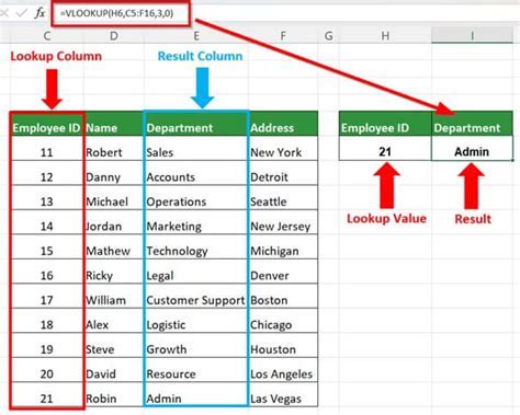
As we delve into the world of Vlookup, it's essential to understand its basic syntax and how it works. The Vlookup function takes four arguments: the value you want to search for, the range of cells where the value is located, the column number that contains the value you want to return, and an optional range lookup argument. By combining these elements, you can create powerful formulas that simplify your data analysis tasks. Now, let's explore five ways to use the Vlookup function, along with examples and explanations to help you get the most out of this valuable tool.

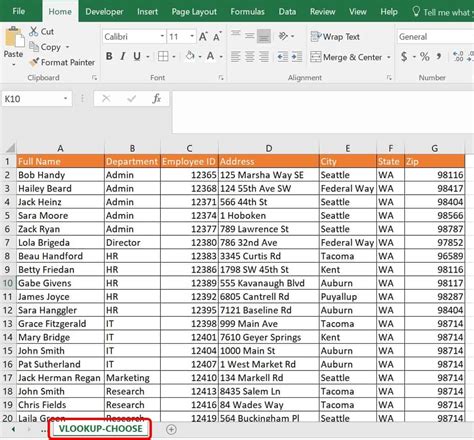
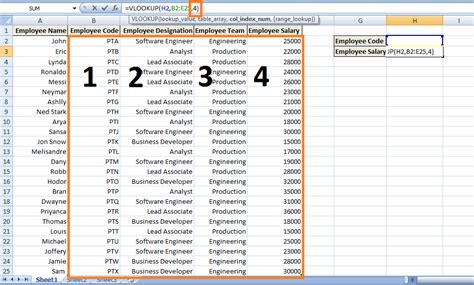
Basic Vlookup Function

The basic Vlookup function is the most straightforward way to use this tool. It involves searching for a value in a table and returning a corresponding value from another column. For instance, suppose you have a table with employee names in one column and their respective job titles in another. You can use the Vlookup function to find an employee's job title based on their name. This is achieved by using the formula =VLOOKUP(lookup value, table array, col index num, [range lookup]), where the lookup value is the employee's name, the table array is the range of cells containing the employee data, the col index num is the column number that contains the job titles, and the range lookup is an optional argument that specifies whether you want an exact match or an approximate match.

Example of Basic Vlookup

To illustrate this concept, let's consider an example. Suppose you have the following table:

Employee Name	Job Title
John Smith	Manager
Jane Doe	Sales Representative
Bob Johnson	IT Specialist

If you want to find John Smith's job title, you can use the formula =VLOOKUP("John Smith", A1:B3, 2, FALSE), where A1:B3 is the range of cells containing the employee data, and 2 is the column number that contains the job titles. The result will be "Manager".

Vlookup with Multiple Criteria

In some cases, you may need to search for a value based on multiple criteria. While the Vlookup function itself does not support multiple criteria, you can use it in combination with other functions, such as the INDEX and MATCH functions, to achieve this result. For example, suppose you have a table with employee names, job titles, and departments, and you want to find an employee's job title based on their name and department. You can use the formula =INDEX(C:C, MATCH(1, (A:A="John Smith") * (B:B="Sales"), 0)), where C:C is the column containing the job titles, A:A is the column containing the employee names, and B:B is the column containing the departments.

Example of Vlookup with Multiple Criteria

To illustrate this concept, let's consider an example. Suppose you have the following table:

Employee Name	Department	Job Title
John Smith	Sales	Sales Representative
Jane Doe	Marketing	Marketing Manager
Bob Johnson	IT	IT Specialist

If you want to find John Smith's job title in the Sales department, you can use the formula =INDEX(C:C, MATCH(1, (A:A="John Smith") * (B:B="Sales"), 0)), where C:C is the column containing the job titles, A:A is the column containing the employee names, and B:B is the column containing the departments. The result will be "Sales Representative".

Vlookup with Approximate Match

In some cases, you may need to search for a value based on an approximate match. The Vlookup function allows you to do this by setting the range lookup argument to TRUE. For example, suppose you have a table with employee names and their respective salaries, and you want to find an employee's salary based on their name, but the name is not spelled exactly as it appears in the table. You can use the formula =VLOOKUP("John Smit", A1:B3, 2, TRUE), where A1:B3 is the range of cells containing the employee data, and 2 is the column number that contains the salaries.

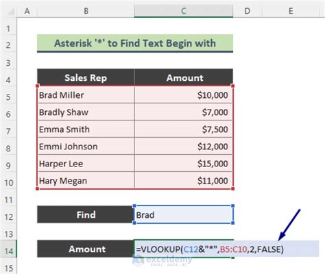
Example of Vlookup with Approximate Match

To illustrate this concept, let's consider an example. Suppose you have the following table:

Employee Name	Salary
John Smith	50000
Jane Doe	60000
Bob Johnson	70000

If you want to find John Smit's salary, you can use the formula =VLOOKUP("John Smit", A1:B3, 2, TRUE), where A1:B3 is the range of cells containing the employee data, and 2 is the column number that contains the salaries. The result will be 50000, assuming that "John Smit" is close enough to "John Smith" to be considered an approximate match.

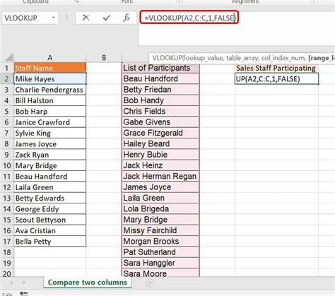
Vlookup with Error Handling

In some cases, the Vlookup function may return an error if the value you are searching for is not found in the table. To handle this situation, you can use the IFERROR function in combination with the Vlookup function. For example, suppose you have a table with employee names and their respective job titles, and you want to find an employee's job title based on their name, but the name is not found in the table. You can use the formula =IFERROR(VLOOKUP("John Smith", A1:B3, 2, FALSE), "Not Found"), where A1:B3 is the range of cells containing the employee data, and 2 is the column number that contains the job titles.

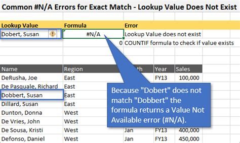
Example of Vlookup with Error Handling

To illustrate this concept, let's consider an example. Suppose you have the following table:

Employee Name	Job Title
John Smith	Manager
Jane Doe	Sales Representative
Bob Johnson	IT Specialist

If you want to find John Smit's job title, you can use the formula =IFERROR(VLOOKUP("John Smit", A1:B3, 2, FALSE), "Not Found"), where A1:B3 is the range of cells containing the employee data, and 2 is the column number that contains the job titles. The result will be "Not Found", since "John Smit" is not found in the table.

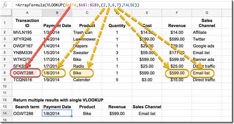
Vlookup with Array Formula

In some cases, you may need to use the Vlookup function with an array formula to search for multiple values at once. For example, suppose you have a table with employee names and their respective job titles, and you want to find the job titles of multiple employees based on their names. You can use the formula =VLOOKUP(A2:A3, B:C, 2, FALSE), where A2:A3 is the range of cells containing the employee names, and B:C is the range of cells containing the employee data.

Example of Vlookup with Array Formula

To illustrate this concept, let's consider an example. Suppose you have the following table:

Employee Name	Job Title
John Smith	Manager
Jane Doe	Sales Representative
Bob Johnson	IT Specialist

If you want to find the job titles of John Smith and Jane Doe, you can use the formula =VLOOKUP(A2:A3, B:C, 2, FALSE), where A2:A3 is the range of cells containing the employee names, and B:C is the range of cells containing the employee data. The result will be an array of job titles, {Manager, Sales Representative}.

Vlookup Image Gallery

What is the Vlookup function in Excel?

+

The Vlookup function is a powerful tool in Microsoft Excel that allows users to search for and retrieve data from a table based on a specific value.

How do I use the Vlookup function with multiple criteria?

+

To use the Vlookup function with multiple criteria, you can combine it with other functions, such as the INDEX and MATCH functions.

What is the difference between an exact match and an approximate match in Vlookup?

+

An exact match in Vlookup requires the value to be searched to match exactly with the value in the table, while an approximate match allows for some flexibility in the match.

How do I handle errors in the Vlookup function?

+

To handle errors in the Vlookup function, you can use the IFERROR function in combination with the Vlookup function.

Can I use the Vlookup function with an array formula?

+

Yes, you can use the Vlookup function with an array formula to search for multiple values at once.

In conclusion, the Vlookup function is a powerful tool in Microsoft Excel that can be used in a variety of ways to search for and retrieve data from a table. By mastering the different ways to use the Vlookup function, you can significantly enhance your productivity and data analysis capabilities. Whether you are a student, a professional, or an entrepreneur, understanding how to use the Vlookup function is essential for making informed decisions in today's data-driven world. We encourage you to practice using the Vlookup function and to explore its many applications in your work and personal projects. With its versatility and power, the Vlookup function is an indispensable tool for anyone working with data in Microsoft Excel.