Highlight Rows In Google Sheets

Highlighting rows in Google Sheets can be a useful way to draw attention to specific data, make it easier to read, or even automate tasks based on conditions. Google Sheets offers several methods to highlight rows, including using formulas, conditional formatting, and scripts. Whether you're looking to highlight rows based on specific values, dates, or other conditions, Google Sheets provides the tools you need.

The importance of highlighting rows cannot be overstated, especially in large datasets where key information might be buried under a sea of numbers and text. By visually distinguishing certain rows, you can quickly identify trends, outliers, or critical data points without having to manually sift through each row. This not only saves time but also reduces the likelihood of human error.

For individuals and businesses alike, the ability to highlight rows in Google Sheets can be a game-changer. It can help in creating more effective reports, tracking inventory, managing projects, and analyzing customer behavior, among other applications. Moreover, because Google Sheets is a cloud-based application, highlighted rows can be shared in real-time with colleagues or stakeholders, facilitating collaboration and decision-making.

Using Conditional Formatting to Highlight Rows

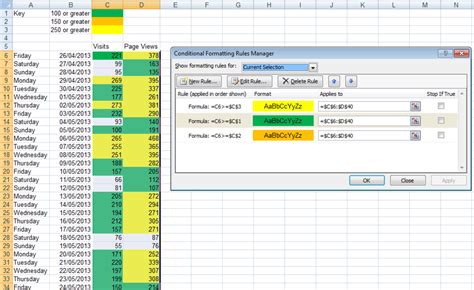
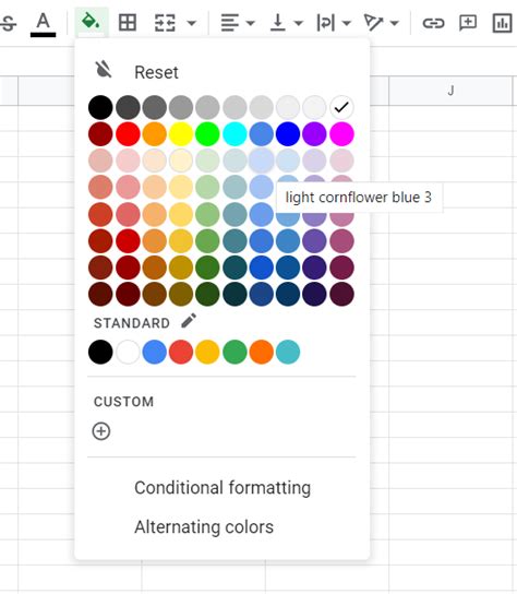
Conditional formatting is one of the most powerful tools in Google Sheets for highlighting rows. It allows you to apply formatting to cells based on their values or formulas. To highlight rows using conditional formatting, follow these steps:

1. Select the range of cells you want to apply the formatting to.
2. Go to the "Format" tab in the menu.
3. Click on "Conditional formatting."
4. In the format cells if dropdown, choose the condition you want to apply (e.g., "Custom formula is").
5. Enter your formula or select a pre-defined rule.
6. Click on the "Done" button.

For example, if you want to highlight rows where the value in column A is greater than 10, you would use the formula =A1>10 and apply it to the entire range of cells you're interested in.

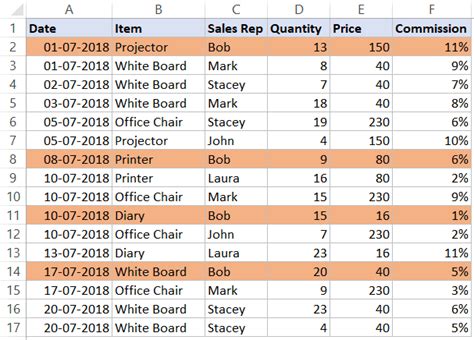
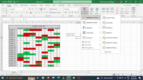
Highlighting Rows Based on Specific Values

Sometimes, you might want to highlight rows based on specific values in a column. This can be achieved through conditional formatting as well. Here’s how:

1. Select the column you want to apply the rule to.
2. Open the conditional formatting sidebar.
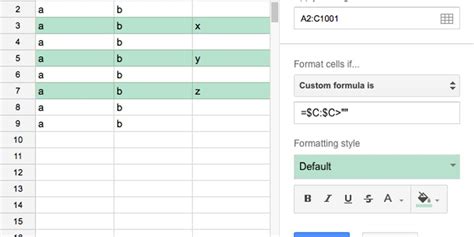
3. Choose "Format cells if" and then select "Custom formula is".
4. Use a formula like =REGEXMATCH(A1, "specificvalue") to match the specific value in column A.
5. Apply the formatting you want and click "Done".

This method is particularly useful for identifying rows that contain specific keywords or phrases.

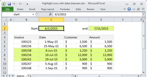
Highlighting Rows with Formulas

Formulas can also be used to highlight rows dynamically based on conditions. For instance, if you want to highlight rows where the sum of values in columns B and C is greater than 100, you can use a formula like =B1+C1>100 in the conditional formatting rule.

To apply a formula for highlighting rows:

1. Select your data range.
2. Go to the conditional formatting option.
3. Choose "Custom formula is".
4. Enter your formula, ensuring it refers to the top-left cell of your selected range (e.g., =B1+C1>100).
5. Choose your formatting and apply.

This approach allows for complex conditions and is highly customizable.

Using Google Apps Script to Highlight Rows

For more advanced users, Google Apps Script offers a programmatic way to highlight rows based on virtually any condition. You can write scripts to automate the highlighting process, which can be especially useful for repetitive tasks or complex logic that conditional formatting cannot handle.

To get started with Google Apps Script for highlighting rows:

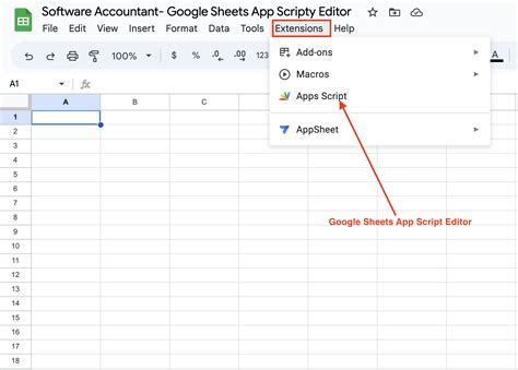
1. Open your Google Sheet.
2. Click on "Tools" > "Script editor".
3. Write your script using JavaScript, specifying the conditions under which rows should be highlighted.
4. Use the getRange() and setBackground() methods to apply highlighting to specific rows.
5. Save and run your script.

Example Script

function highlightRows() {
  var sheet = SpreadsheetApp.getActiveSheet();
  var dataRange = sheet.getDataRange();
  var values = dataRange.getValues();
  
  for (var i = 0; i < values.length; i++) {
    if (values[i][0] > 10) { // Highlight row if value in column A is greater than 10
      sheet.getRange(i + 1, 1, 1, dataRange.getLastColumn()).setBackground("yellow");
    }
  }
}

This script highlights rows where the value in the first column is greater than 10.

Best Practices for Highlighting Rows

When highlighting rows in Google Sheets, keep the following best practices in mind:

• Use Consistent Formatting: Ensure that your highlighting is consistent throughout your sheet to avoid confusion.
• Keep it Simple: Avoid over-highlighting, as this can make your sheet look cluttered and difficult to read.
• Use Conditional Formatting Wisely: Conditional formatting rules can slow down your sheet if overused. Keep the number of rules to a minimum.
• Test Your Formulas: Before applying highlighting formulas to large datasets, test them on a small sample to ensure they work as expected.

Gallery of Highlighting Rows in Google Sheets

Highlighting Rows Image Gallery

How do I highlight rows in Google Sheets based on a condition?

+

To highlight rows in Google Sheets based on a condition, use conditional formatting. Select your range, go to the "Format" tab, click on "Conditional formatting," and choose your condition or enter a custom formula.

Can I highlight rows using Google Apps Script?

+

Yes, Google Apps Script can be used to highlight rows programmatically. You can write a script to apply highlighting based on specific conditions or complex logic that cannot be achieved with conditional formatting alone.

How do I avoid slowing down my Google Sheet with too many conditional formatting rules?

+

To avoid slowing down your Google Sheet, limit the number of conditional formatting rules. Apply rules only where necessary, and consider using Google Apps Script for complex or dynamic highlighting tasks.

In conclusion, highlighting rows in Google Sheets is a versatile tool that can significantly enhance your data analysis and presentation capabilities. Whether through conditional formatting, formulas, or Google Apps Script, there's a method to suit every need. By following best practices and exploring the various options available, you can unlock the full potential of your data and make more informed decisions. If you have any further questions or need more detailed guidance on specific aspects of highlighting rows, feel free to ask in the comments below. Sharing your experiences or tips on how you use highlighting in Google Sheets can also be beneficial for others, so don't hesitate to share.