5 Ways To Link Cells

Linking cells in a spreadsheet is a fundamental skill that can significantly enhance your data management and analysis capabilities. Whether you're using Google Sheets, Microsoft Excel, or another spreadsheet program, understanding how to link cells is crucial for creating dynamic and interactive worksheets. This article will delve into the importance of linking cells, the different methods to do so, and provide practical examples to help you master this essential skill.

Effective data analysis and presentation often require combining data from multiple cells or worksheets. By linking cells, you can create formulas that automatically update when the source data changes, ensuring that your calculations and charts always reflect the latest information. This feature is particularly useful in financial planning, scientific research, and business intelligence, where data is constantly evolving.

The ability to link cells also enables the creation of complex models and simulations. For instance, in a budgeting spreadsheet, you might link cells to calculate the total cost of expenses based on individual line items. As you update the costs of specific expenses, the total automatically adjusts, providing a real-time overview of your budget. This dynamic capability makes spreadsheet software an indispensable tool for professionals and individuals alike.

Understanding Cell References

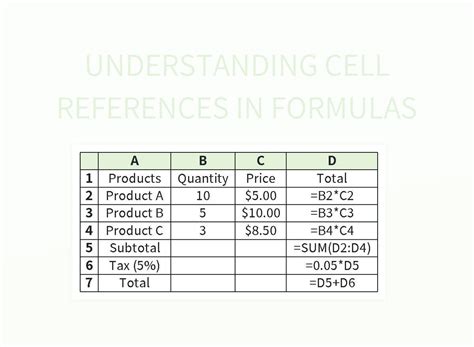
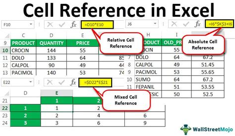
Before diving into the methods of linking cells, it's essential to understand cell references. A cell reference identifies a cell or a range of cells in a spreadsheet. There are two types of cell references: relative and absolute. Relative references change when a formula is copied to another cell, while absolute references remain the same. Understanding the difference between these reference types is crucial for linking cells effectively.

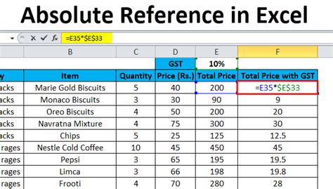
Method 1: Using Absolute References

Absolute references are denoted by a dollar sign ($). When you use an absolute reference in a formula, the column letter and row number are fixed. For example, $A$1 refers to the cell in column A, row 1, and this reference will not change if the formula is copied to another cell. Absolute references are useful when you want to link cells in different parts of your spreadsheet but ensure that the reference to a specific cell or range remains constant.

Steps to Use Absolute References

To use absolute references, follow these steps:

Select the cell where you want to enter the formula.
Type the equals sign (=) to start the formula.
Click on the cell you want to reference, or type the cell reference manually, including the dollar signs for absolute references (e.g., $A$1).
Complete the formula as needed and press Enter.

Method 2: Using Relative References

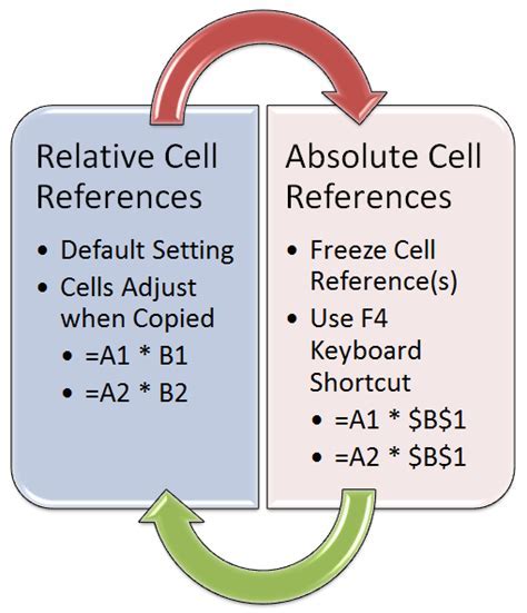
Relative references, on the other hand, do not use the dollar sign. When you copy a formula with a relative reference to another cell, the reference adjusts based on the relative position of the cells. For example, if you have a formula =A1 in cell B1 and you copy it to cell B2, the formula in B2 becomes =A2. Relative references are convenient for applying the same formula across a range of cells where the relative position of the data is consistent.

Steps to Use Relative References

Using relative references is straightforward:

Select the cell for your formula.
Start the formula with the equals sign (=).
Click on the cell you want to reference or type the cell reference without dollar signs (e.g., A1).
Complete your formula and press Enter.

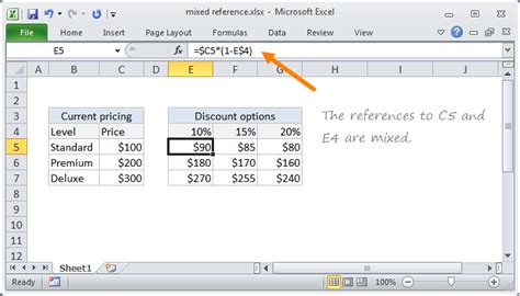
Method 3: Using Mixed References

Mixed references combine elements of both absolute and relative references. You can fix either the column or the row by using the dollar sign before either the column letter or the row number, but not both. For example, $A1 fixes the column but allows the row to change, while A$1 fixes the row but allows the column to change. Mixed references are useful in scenarios where you need to apply a formula across a range of cells but want to keep either the column or row reference constant.

Steps to Use Mixed References

To use mixed references:

Determine whether you need to fix the column or the row.
Start your formula with the equals sign (=).
If fixing the column, use $ before the column letter (e.g., $A1). If fixing the row, use $ after the row number (e.g., A$1).
Complete the formula and press Enter.

Method 4: Linking Cells Across Worksheets

Linking cells across different worksheets within the same spreadsheet is also possible. This is particularly useful for compiling data from multiple sources into a summary sheet. To link cells across worksheets, you specify the worksheet name followed by an exclamation mark (!) and then the cell reference. For example, =Sheet1!A1 references cell A1 in Sheet1.

Steps to Link Cells Across Worksheets

To link cells across worksheets:

Ensure the worksheets are in the same spreadsheet file.
Select the cell where you want to enter the formula.
Type the equals sign (=) to start the formula.
Type the name of the worksheet you want to reference, followed by an exclamation mark (!), and then the cell reference (e.g., =Sheet2!A1).
Press Enter to complete the formula.

Method 5: Linking Cells Across Different Spreadsheet Files

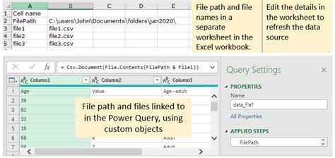
In some cases, you may need to link cells across different spreadsheet files. This can be achieved by using an external reference. The syntax for an external reference includes the file path, the file name, the worksheet name, and the cell reference, all separated by exclamation marks. For example, ='C:[Workbook1.xlsx]Sheet1'!$A$1 references cell A1 in Sheet1 of Workbook1.xlsx located on the C drive.

Steps to Link Cells Across Different Spreadsheet Files

To link cells across different spreadsheet files:

Open both the source and destination spreadsheet files.
In the destination file, select the cell for the formula.
Start the formula with the equals sign (=).
Type the file path and name of the source file in single quotes, followed by the worksheet name and cell reference, using exclamation marks to separate these elements (e.g., ='C:[Workbook2.xlsx]Sheet2'!A1).
Press Enter to complete the formula.

Linking Cells Image Gallery

What is the difference between absolute and relative cell references?

Absolute references ($A$1) do not change when a formula is copied, while relative references (A1) adjust based on the new cell's position.

How do I link cells across different worksheets in the same spreadsheet?

Use the worksheet name followed by an exclamation mark and the cell reference (e.g., =Sheet1!A1).

Can I link cells across different spreadsheet files?

Yes, by using an external reference that includes the file path, file name, worksheet name, and cell reference (e.g., ='C:\[Workbook1.xlsx]Sheet1'!$A$1).

In conclusion, mastering the art of linking cells is a fundamental aspect of working with spreadsheets. Whether you're using absolute, relative, or mixed references, or linking across worksheets or files, understanding how to create dynamic and interactive formulas can significantly enhance your productivity and data analysis capabilities. By following the methods and examples outlined in this article, you'll be well on your way to becoming proficient in linking cells and unlocking the full potential of your spreadsheet software. Remember, practice makes perfect, so don't hesitate to experiment and explore the various ways you can link cells to achieve your goals. Share your experiences, tips, and questions in the comments below, and help create a community of spreadsheet enthusiasts who can learn from and support each other.