Add Data Labels In Excel

Data labels are a crucial aspect of data visualization in Excel, allowing users to quickly understand the values represented by their charts and graphs. By adding data labels to your Excel charts, you can enhance the readability and comprehension of your data, making it easier for audiences to grasp complex information at a glance. In this article, we will delve into the importance of data labels, how to add them to your Excel charts, and provide tips on customizing them for maximum effectiveness.

The ability to clearly communicate data insights is fundamental in today's data-driven world. Whether you're presenting sales figures, website traffic, or scientific findings, data labels can significantly improve the clarity of your charts. They provide immediate context to the data points on your graph, eliminating the need for viewers to hover over each point or refer to a legend. This feature is particularly useful in presentations, reports, and dashboards where concise and clear communication is key.

Excel, being one of the most widely used spreadsheet programs, offers robust features for creating and customizing data labels. The process of adding data labels is straightforward and can be accomplished in a few steps. First, you need to select the chart to which you want to add data labels. This can be any type of chart, from a simple column chart to a more complex combination chart. Once your chart is selected, you can navigate to the "Chart Design" or "Chart Tools" tab on the ribbon, depending on your version of Excel. Here, you'll find the option to add data labels.

Adding Data Labels to Your Excel Chart

To add data labels, follow these steps:

• Select your chart by clicking on it.
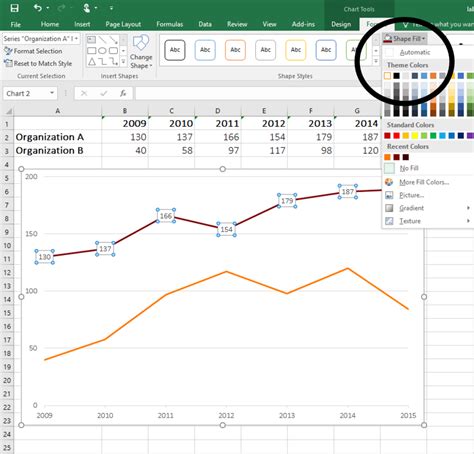
• Go to the "Chart Design" tab.
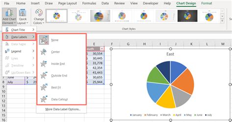
• Click on "Add Chart Element" and select "Data Labels" from the drop-down menu.
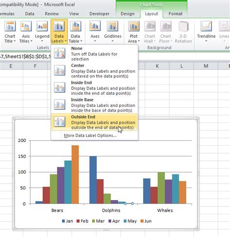
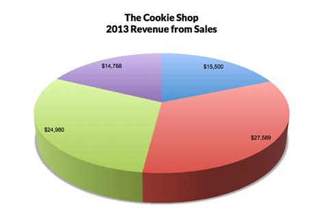
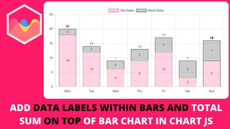
• Choose where you want the data labels to be placed, such as "Center" for pie charts or "Inside End" for bar charts.

Customizing Data Labels

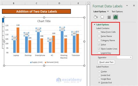
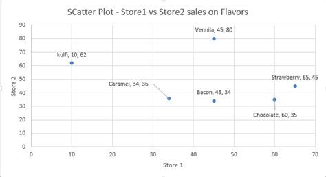
Customization is a powerful feature in Excel that allows you to tailor your data labels to your specific needs. You can change the format of the labels, adjust their position, and even add additional information such as the data point's percentage value in a pie chart. To customize data labels, select the data labels on your chart, and then use the options available in the "Format Data Labels" pane. Here, you can check boxes to include series name, category name, and value, among other options. You can also use the "Number" section to change how the values are displayed, such as showing them as percentages or currency.

Benefits of Using Data Labels

The benefits of using data labels are multifaceted:

• Enhanced Readability: Data labels make your charts more understandable by providing direct values.
• Improved Precision: Viewers can see the exact values without needing to guess or use a legend.
• Flexibility: Excel offers various customization options to fit different types of data and presentation styles.

Common Challenges and Solutions

While data labels are incredibly useful, there are common challenges users face, such as overlapping labels or labels being too large for the chart. To address these issues, you can adjust the label's position, rotate the text, or use the "Format Data Labels" options to select which labels to show. For instance, showing only the top n values can help declutter your chart.

Advanced Techniques for Data Labels

For more complex data visualization, Excel allows for advanced techniques such as using formulas within data labels. This can be particularly useful for adding dynamic text or calculations directly to your labels. To use a formula in a data label, you might need to use a combination of Excel functions and the "Format Data Labels" pane to reference cells or calculations.

Best Practices for Data Label Usage

Best practices include:

• Use Them Sparingly: Too many data labels can clutter your chart. Use them only where necessary.
• Customize for Clarity: Adjust font sizes, colors, and positions to ensure labels are easy to read.
• Consistency: Apply similar formatting across all your charts for a cohesive look.

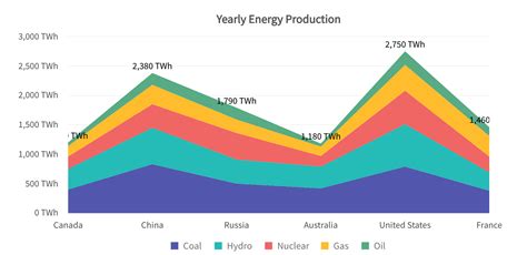
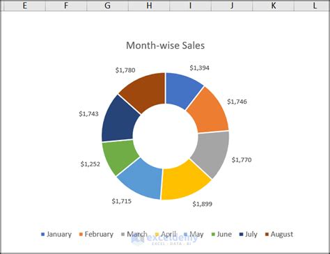
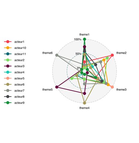
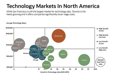
Gallery of Data Label Examples

Data Label Image Gallery

How do I add data labels to a chart in Excel?

+

To add data labels, select your chart, go to the "Chart Design" tab, click on "Add Chart Element," and choose "Data Labels" from the drop-down menu.

Can I customize the appearance of data labels in Excel?

+

Yes, you can customize data labels by selecting them, then using the "Format Data Labels" pane to change their format, position, and what they display.

How do I resolve overlapping data labels in Excel charts?

+

To resolve overlapping labels, you can adjust their position, rotate the text, or show only the top n values to declutter your chart.

In conclusion, data labels are a powerful tool in Excel that can significantly enhance the effectiveness of your charts and graphs. By understanding how to add, customize, and use data labels strategically, you can communicate complex data insights more clearly and engagingly. Whether you're a seasoned Excel user or just starting out, mastering the use of data labels can elevate your data visualization skills, making your presentations and reports more impactful and easier to understand. We invite you to share your experiences and tips on using data labels in Excel, and to explore how this feature can be applied in various contexts to improve data communication.