5 Ways Excel Conditional Formatting

The importance of data analysis and visualization in today's fast-paced business world cannot be overstated. With the vast amounts of data being generated every day, it's crucial to have the right tools to make sense of it all. One such tool is Microsoft Excel, a powerful spreadsheet software that offers a wide range of features to help users analyze and visualize data. One of the most useful features in Excel is conditional formatting, which allows users to highlight cells based on specific conditions. In this article, we'll explore five ways to use Excel conditional formatting to take your data analysis to the next level.

Conditional formatting is a powerful tool that can help users quickly identify trends, patterns, and outliers in their data. By applying different formats to cells based on specific conditions, users can make their data more visual and easier to understand. Whether you're a financial analyst, a marketing manager, or a business owner, conditional formatting can help you make better decisions by providing a clearer picture of your data.

With the increasing amount of data being generated every day, it's becoming more and more important to have the right tools to analyze and visualize it. Excel conditional formatting is one such tool that can help users make sense of their data. By applying different formats to cells based on specific conditions, users can quickly identify trends, patterns, and outliers in their data. In this article, we'll explore five ways to use Excel conditional formatting to take your data analysis to the next level.

Introduction to Conditional Formatting

Conditional formatting is a feature in Excel that allows users to highlight cells based on specific conditions. This can be done using a variety of formats, including colors, icons, and data bars. By applying different formats to cells based on specific conditions, users can make their data more visual and easier to understand. Conditional formatting can be used to highlight cells that meet specific criteria, such as cells that contain a specific value or cells that fall within a specific range.

Types of Conditional Formatting

There are several types of conditional formatting that can be used in Excel, including: * Highlight cells rules: This type of formatting allows users to highlight cells based on specific conditions, such as cells that contain a specific value or cells that fall within a specific range. * Top/Bottom rules: This type of formatting allows users to highlight cells that are in the top or bottom of a range, such as the top 10% or bottom 20%. * Data bars: This type of formatting allows users to display data bars in cells, which can be used to compare values across a range. * Color scales: This type of formatting allows users to display color scales in cells, which can be used to compare values across a range. * Icon sets: This type of formatting allows users to display icons in cells, which can be used to indicate specific conditions, such as trends or patterns.

5 Ways to Use Conditional Formatting

Now that we've covered the basics of conditional formatting, let's explore five ways to use it to take your data analysis to the next level.

1. Highlighting Cells Based on Specific Conditions

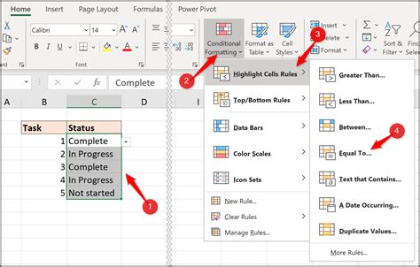
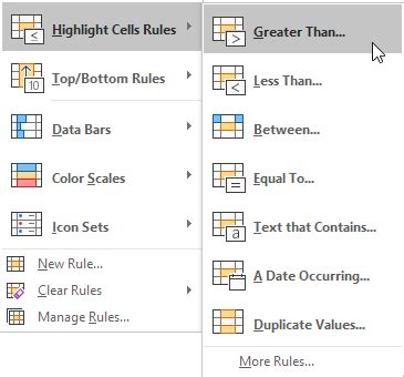
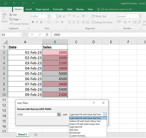
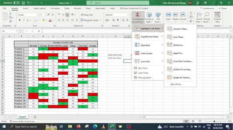
One of the most common uses of conditional formatting is to highlight cells based on specific conditions. For example, you might want to highlight cells that contain a specific value, such as a specific product name or a specific region. To do this, you can use the "Highlight cells rules" feature in Excel. Simply select the range of cells that you want to format, go to the "Home" tab, and click on "Conditional Formatting." Then, select "Highlight cells rules" and choose the condition that you want to apply.

2. Identifying Trends and Patterns

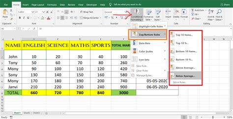
Conditional formatting can also be used to identify trends and patterns in your data. For example, you might want to highlight cells that are above or below a certain threshold, or cells that are increasing or decreasing over time. To do this, you can use the "Top/Bottom rules" feature in Excel. Simply select the range of cells that you want to format, go to the "Home" tab, and click on "Conditional Formatting." Then, select "Top/Bottom rules" and choose the condition that you want to apply.

3. Visualizing Data with Data Bars

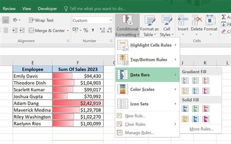
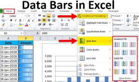
Data bars are a type of conditional formatting that can be used to display data bars in cells. This can be useful for comparing values across a range, such as sales data or customer satisfaction ratings. To apply data bars, simply select the range of cells that you want to format, go to the "Home" tab, and click on "Conditional Formatting." Then, select "Data bars" and choose the type of data bar that you want to apply.

4. Using Color Scales to Compare Values

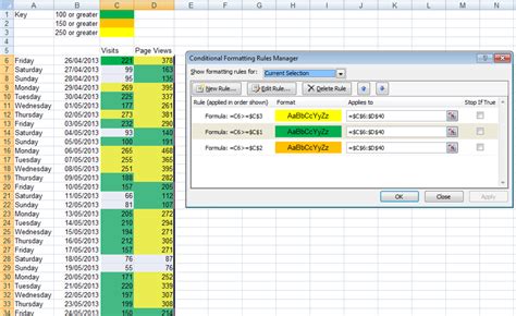
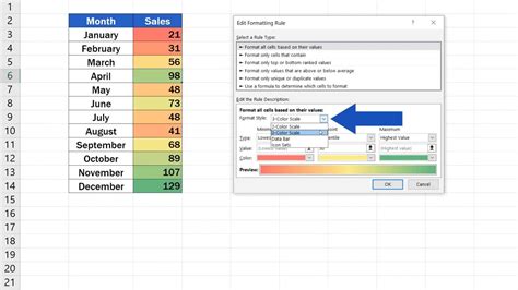
Color scales are another type of conditional formatting that can be used to compare values across a range. This can be useful for identifying trends and patterns in your data, such as changes in sales data or customer satisfaction ratings over time. To apply color scales, simply select the range of cells that you want to format, go to the "Home" tab, and click on "Conditional Formatting." Then, select "Color scales" and choose the type of color scale that you want to apply.

5. Using Icon Sets to Indicate Specific Conditions

Icon sets are a type of conditional formatting that can be used to display icons in cells. This can be useful for indicating specific conditions, such as trends or patterns in your data. To apply icon sets, simply select the range of cells that you want to format, go to the "Home" tab, and click on "Conditional Formatting." Then, select "Icon sets" and choose the type of icon set that you want to apply.

Best Practices for Using Conditional Formatting

Now that we've covered the basics of conditional formatting, let's explore some best practices for using it effectively.

Use conditional formatting to highlight important trends and patterns in your data.
Use different types of conditional formatting to compare values across a range.
Use icon sets to indicate specific conditions, such as trends or patterns in your data.
Use data bars to display data bars in cells, which can be useful for comparing values across a range.
Use color scales to compare values across a range, which can be useful for identifying trends and patterns in your data.

Common Mistakes to Avoid

When using conditional formatting, there are several common mistakes to avoid. These include: * Overusing conditional formatting, which can make your data difficult to read. * Using too many different types of conditional formatting, which can be confusing. * Not using conditional formatting consistently, which can make it difficult to compare values across a range. * Not testing your conditional formatting rules, which can lead to errors.

Conclusion and Next Steps

In conclusion, conditional formatting is a powerful tool in Excel that can be used to highlight important trends and patterns in your data. By using the different types of conditional formatting, such as highlight cells rules, top/bottom rules, data bars, color scales, and icon sets, you can make your data more visual and easier to understand. Remember to use conditional formatting consistently and test your rules to avoid errors.

Final Thoughts

Conditional formatting is a powerful tool that can help you take your data analysis to the next level. By using the different types of conditional formatting, you can make your data more visual and easier to understand. Remember to use conditional formatting consistently and test your rules to avoid errors. With practice and experience, you can become proficient in using conditional formatting to analyze and visualize your data.

Excel Conditional Formatting Image Gallery

What is conditional formatting in Excel?

Conditional formatting is a feature in Excel that allows users to highlight cells based on specific conditions.

What are the different types of conditional formatting in Excel?

The different types of conditional formatting in Excel include highlight cells rules, top/bottom rules, data bars, color scales, and icon sets.

How do I apply conditional formatting in Excel?

To apply conditional formatting in Excel, select the range of cells that you want to format, go to the "Home" tab, and click on "Conditional Formatting." Then, select the type of conditional formatting that you want to apply and choose the condition that you want to use.

What are some best practices for using conditional formatting in Excel?

Some best practices for using conditional formatting in Excel include using it to highlight important trends and patterns in your data, using different types of conditional formatting to compare values across a range, and testing your rules to avoid errors.

How do I avoid common mistakes when using conditional formatting in Excel?

To avoid common mistakes when using conditional formatting in Excel, make sure to use it consistently, test your rules, and avoid overusing it. Additionally, make sure to use the correct type of conditional formatting for your data and avoid using too many different types of conditional formatting.

We hope this article has provided you with a comprehensive understanding of how to use Excel conditional formatting to take your data analysis to the next level. Whether you're a beginner or an experienced user, conditional formatting is a powerful tool that can help you make better decisions by providing a clearer picture of your data. If you have any questions or comments, please don't hesitate to reach out. Share this article with your friends and colleagues who may benefit from learning more about Excel conditional formatting.